Unit 2 Technology and incentives
2.4 Firms, technology, and production
- technology
- The description of a process that uses a set of materials and other inputs, including the work of people and machines, to produce an output.
Firms own or rent capital goods—such as buildings and equipment—and employ workers to produce and sell goods and services. An important decision for a firm is its choice of production technology: the process that it will use to convert a set of inputs—such as raw materials, and work done by people and machinery—into output that it can sell. Having chosen a technology, it will also need to decide on the amount of inputs to employ, which will determine how much output it can produce.
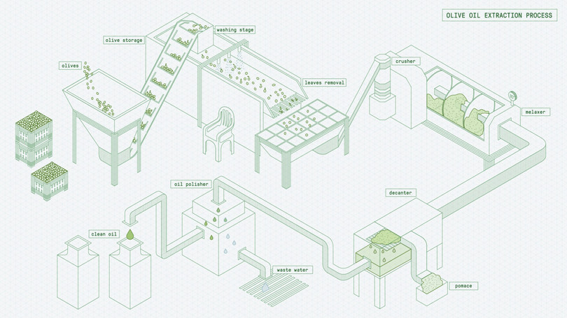
For example, in the production of olive oil, the olives must be graded, washed, milled to remove the stones, mashed to a paste, and pressed to extract oil and water. Finally, the oil is separated from the water and canned or bottled. For thousands of years it was produced using simple technologies in which most of the process was carried out by hand, using a pestle and mortar to mash the olives, and heavy stones to press them. The inputs were raw materials (olives and water); capital (pestle and mortar, stones); and labour. It was a labour-intensive technology: 2,000 olives had to be combined with many hours of hard work to produce a litre of oil.
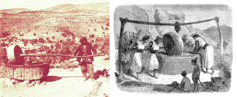
A labour-intensive technology for producing olive oil.
A capital-intensive olive technology.
- factor of production
- Any input into a production process is called a factor of production. Factors of production may include labour, machinery and equipment (usually referred to as capital), land, energy, and raw materials.
- production function
- A production function is a graphical or mathematical description of the relationship between the quantities of the inputs to a production process and the amount of output produced. When used to represent output in the whole economy, it is described as an aggregate production function.
The technology used in modern commercial production employs less labour and more capital and energy. The inputs, or factors of production, are raw materials, labour, capital goods (milling, mashing, and pressing machines), and energy to operate the machines.
A technology can be represented by a production function: a relationship that tells us how much output it will produce, given the amounts of inputs used. The technology described in Section 1.6 produces agricultural output, Y, using labour and land. Since the amount of land is assumed to be constant, we write the production function as Y = f(X), where X is the number of farmers. This function is shown in Figure 1.8b.
In the case of olive oil, suppose that N is the number of workers employed, M is the number of machines, and E is the amount of energy used per day. Then we can summarize the technology using a production function for the amount of olive oil produced per day, Y:
\[Y = \text{f}(M, N, E)\]This expression is just a shorthand way of saying ‘the daily output of oil, Y, depends on (or is a function of) the amounts of the inputs, N, M, and E, that the firm chooses to use’. We have ignored raw materials, assuming that the number of olives required is automatically determined by the volume of oil to be produced.
Figure 2.3 describes a hypothetical technology for olive oil. Imagine that there are three machines (for milling, mashing, and pressing). With the help of a single worker to operate them, and 80 kWh of energy, they can produce 50 litres of olive oil per day. If the firm wants to produce more, it needs more machines, workers, and energy. The table shows how much output is produced, for different combinations of factors of production.
| Number of machines, M | Number of workers, N | Amount of energy, E (kWh) | Output, Y (litres) |
|---|---|---|---|
| 3 | 1 | 80 | 50 |
| 6 | 2 | 160 | 100 |
| 9 | 3 | 240 | 150 |
| 12 | 4 | 320 | 200 |
Figure 2.3 A fixed-proportions technology for making olive oil.
- fixed-proportions technology
- A technology that requires inputs in fixed proportions to each other. To increase the amount of output, all inputs must be increased by the same percentage so that they remain in the same fixed proportions to each other.
- constant returns to scale
- When production exhibits constant returns to scale, increasing all of the inputs to a production process by the same proportion increases output by the same proportion. The shape of a firm’s long-run average cost curve depends both on returns to scale in production and the effect of scale on the prices it pays for its inputs. See also: increasing returns to scale, decreasing returns to scale.
This technology is simple to describe, for two reasons. First, it requires inputs in fixed proportions: for every three machines, one worker, and 80 kWh of energy are needed. With a fixed-proportions technology there is no point in increasing one input without increasing the others. For example, if you have six machines, you can’t make them run any faster even if you add a third worker or more energy: output will remain at 100 litres.
Secondly, it has constant returns to scale: if you double the inputs, the amount of output doubles; similarly a 50% increase in inputs (from the second row of the table to the third) increases output by 50%. (So you could easily add more rows to the table.)
We will use technologies with these two properties in Section 2.5, to model the decisions of firms in the Industrial Revolution.
Comparing two technologies
Suppose that a new robotic technology is developed for producing olive oil. This robotic system, which is controlled by one worker and using 400 kWh of energy, can produce 100 litres of olive oil per day. As before, the technology uses inputs in fixed proportions and has constant returns to scale. Daily output is proportional to the number of systems installed. Can we say that the robotic system is better?
A simple way to compare constant-returns technologies is to compare their input requirements for producing a standard amount of output. The table in Figure 2.4 shows the inputs needed for 100 litres of oil per day.
- average product
- The average product of an input is total output divided by the total amount of the input. For example, the average product of a worker (also known as labour productivity) is total output divided by the number of workers employed to produce it.
The fourth column uses these figures to compare the average product of labour: output per worker. With fixed proportions and constant returns, the average product of labour is the same however many workers are employed. For example, output per worker with technology A is 100/2 = 50 litres per day. The last column shows the ratio of the two inputs: it shows that technology B is more energy intensive than technology A.

| Input requirements for 100 litres of olive oil | ||||
|---|---|---|---|---|
| Workers | Energy | Average product of labour | Energy–labour ratio | |
| A: Milling, mashing, and pressing machines | 2 | 160 | 50 | 80 |
| B: Robotic technology | 1 | 400 | 100 | 400 |
Figure 2.4 Summarizing and comparing two fixed-proportions technologies.
The lower panel of Figure 2.4 illustrates this information graphically. In each case, it shows the input requirements for 100 litres of olive oil, and for more output further along the ray from the origin. The slope of each ray corresponds to the energy–labour ratio. The steeper the ray, the more energy-intensive the technology (meaning that the amount of energy—relative to the number of workers—required to produce a given level of output is greater).
The graph shows that neither technology is necessarily better than the other. The average product of labour is higher with technology B, but it uses far more energy. To decide which one to use, the owner of the firm would need to consider the relative costs of the two inputs. This was a key factor in the choice of technology in the Industrial Revolution, as the following sections of this unit will explain.
Question 2.5 Choose the correct answer(s)
Figure 2.4 shows the input requirements for different amounts of olive oil, for two technologies (A and B). Suppose there is a third fixed-proportions technology, C, which requires four workers and 360 units of energy to produce 100 litres of olive oil. Based on this information, read the following statements and choose the correct option(s).
- Since technology C is a fixed-proportions technology with constant returns to scale, we multiply the numbers given by 3 to obtain 4 × 3 = 12 workers and 360 × 3 = 1,080 units of energy.
- The average product of labour of technology C is 100/4 = 25, which is lower than that of technology A and B.
- The energy–labour ratio of technology C is 360/4 = 90, which is between that of technology A (80) and B (400).
- Technology B has a higher average product of labour than technology C, but is also more energy-intensive, so the owner’s choice depends on the relative price of the inputs.
Extension 2.4 Production functions
This extension explains how the fixed-proportions technology used in Unit 2 relates to the more typical production functions in Unit 1 and Unit 5.
The second part explores some mathematical properties of typical production functions like those in Units 1 and 5—in particular, the diminishing average product of labour. This part requires a knowledge of calculus (differentiation).
The Introduction to Mathematical Extensions explains briefly what we mean by calculus and describes the mathematical level, notation, and conventions used.
The fixed-proportions technology discussed in the main part of this section is convenient for analysing some problems, but in practice it is usually possible to vary production by varying one factor but not others. In the example of the agricultural technology in Section 1.6, more grain is produced when the number of farmers increases while the other factor, land, stays constant.
Suppose that it is possible in olive oil production to vary the number of workers relative to the other inputs. With a given amount of machinery and energy, production could be organized more or less intensively, depending on the number of workers. Similarly, with a given workforce, increasing the number of machines might allow an increase in output.
To keep the description of the technology as easy as possible, we will assume that capital (machinery) and energy remain in fixed proportions. So, if you know the amount of energy, you also know the amount of capital (machinery) being used. Then we can think of the production function as a function of two factors:
\[Y = f (N, E)\]The main choices for the firm are the number of workers, \(N\), and the amount of energy, \(E\). Everything else follows automatically. Figure E2.1a shows some possible combinations of the inputs, and the resulting output, for an example of such a production function.
| Number of workers, N | Amount of energy, E (kWh) | Output, Y (litres) | |
|---|---|---|---|
| A | 2 | 200 | 160 |
| B | 2 | 600 | 309 |
| C | 4 | 400 | 320 |
| D | 4 | 800 | 485 |
| F | 6 | 600 | 480 |
| G | 6 | 1000 | 652 |
Figure E2.1a A variable-proportions technology: some combinations of workers, \(N\), and energy, \(E\), and corresponding output, \(Y\).
Like the previous example, this technology has constant returns to scale—as you can verify by comparing lines A, C, and F in the table. But even if we added more combinations, it would not be easy to tell from a table like this how changing one input more than the other affects the amount of oil produced.
We get a better sense of the relationship by plotting the production function using a three-dimensional diagram as in Figure E2.1b. The number of workers, \(N\), is plotted on the (red) x-axis, and the amount of energy, \(E\), on the (green) y-axis. These two axes form the ‘floor’ of the diagram, and each point on the floor corresponds to a different combination of \(N\) and \(E\). Then the corresponding amount of olive oil is given by the distance above the floor, measured on the (blue) z-axis. If we plot the height corresponding to every (\(N\), \(E\)) combination they form a smooth surface—a ‘hill’ that rises as \(N\) and \(E\) increase. The particular points in the table above are marked on the surface.
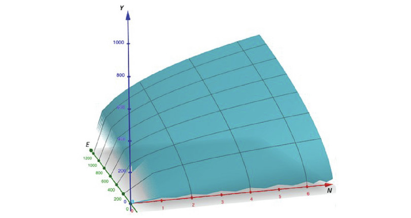
Figure E2.1b A three-dimensional representation of the production function for olive oil: \(Y = f(N, E)\).
This picture shows that, as you would expect, the more labour and energy are used, the more oil is produced. Secondly, if you increase one input while keeping the other constant, output rises—but not as fast as when you increase both inputs together. Imagine yourself climbing the hill from point A, where \(N\) = 2 and \(E\) = 200. Going up to point C (raising both inputs) is a much steeper climb than walking along the line where \(E\) = 200.
A production function with one variable factor
It is often the case that some factors of production can be varied more easily than others.
For example, suppose that a small olive oil producer is currently employing two workers and producing 309 litres per day at point B in Figure E2.1c. It would like to expand, because the price of olive oil has risen, but it cannot raise the funds to buy more machines. So the only way to increase production is to employ extra workers, while keeping its current stock of machinery fixed, and the corresponding energy input at 600. The line in Figure E2.1c through points B and F, corresponding to \(E = 600\), shows how output will change as employment rises. By taking a vertical slice through the hill along this line, as shown in the upper panel of Figure E2.1c, we can obtain a two-dimensional diagram (lower panel).

Figure E2.1c The production function for olive oil when energy is held constant.
The lower panel shows the output of olive oil as a function of labour only, with the other factor, energy, fixed at 600. This production function has a curved (concave) shape similar to the agricultural production function in Section 1.6 (from Figure 1.8c). In both cases, output doesn’t rise proportionally with the number of workers, and this happens because there is a fixed factor (land in Unit 1, energy here). In Figure E2.1c, with a fixed amount of energy and corresponding capital, the number of machines per worker, and hence the amount produced per worker, falls as the number of workers increases.
The production function and the diminishing average product of labour
You will encounter production functions like the one in Figure E2.1c in many economic applications, because inputs such as land, premises, or machinery are often difficult to change, so we need to consider what would happen if the labour input were varied while the other inputs remained constant. Typically, production will increase with more labour, but the ‘fixed’ inputs limit labour productivity and hence lower the amount produced per worker.
In general, if we let \(x\) be the labour input (it could be measured as the number of workers, or their total hours of work) and \(y\) be the amount of output produced (for example, litres of olive oil) we can write the production function as:
\[y = f(x)\]\(f(x)\) could be any function, but if it is to represent a plausible production function, it must have certain properties. First, we can show that if the input is zero, no output is produced, and if the input is greater than zero, output is strictly positive:
\[f(0)=0, \quad f(x)>0 \text{ if } x>0\]Secondly, the function is increasing: that is, as \(x\) increases, so does \(y\). So the slope of the function, which is given by its derivative, is positive. We can write:
\[\frac{dy}{dx}>0\]or equivalently:
\[f'(x)>0\]If the production function has the typical concave shape of the olive oil example, then its slope \(f'(x)\) decreases as \(x\) increases. That is, its second derivative is negative:
\[f''(x)<0\]Figure E2.1d shows the decreasing slope where we have drawn the tangents at two points, B and F, to compare the slopes of the function there. The slope remains positive, but it gets flatter—less positive—as you move to the right.
The average product of labour (APL) is given by total output \(y\) divided by the labour input:
\[\text{APL}=\frac{f(x)}{x}\]
Figure E2.1d The slope of the production function and the average product of labour.
For example, at point B in Figure E2.1d, the firm employs two workers and produces 309 litres of olive oil per day. The APL at B corresponds to the slope of the ray from the origin to point B:
\[\begin{align*} \text{average product of labour} &= \frac{\text{total output}}{\text{total number of workers}} \\ &= \frac{309~ \text{litres}}{2~ \text{workers}} \\ &= 155~ \text{litres per worker} \end{align*}\]- diminishing average product of labour
- A property of a production process in which, as the input of labour is increased, the amount of output per unit of labour (the average product) falls.
The olive oil example, like all production functions with this typical concave shape, has the property of diminishing average product of labour. As we move along it, the production function gets flatter and so the APL falls: at F, average labour productivity has fallen to 480/6 = 80 litres per worker.
We have described the production function using two different slopes: the slope of the function, \(f'(x)\), and the slope of the ray from the origin, \(\text{APL}=f(x)/x\).
We can show that if a production function has the property of diminishing average product, then its slope \(f'(x)\) must always be lower than the APL. By differentiating the average product with respect to \(x\) using the quotient rule, we get:
\[\frac{d\text{APL}}{dx} = \frac{d}{dx}\left(\frac{f(x)}{x}\right) = \left(\frac{xf'(x)-f(x)}{x^2}\right)\]If the average product is diminishing, this expression must be negative:
\[\begin{align*} \frac{d\text{APL}}{dx} < 0 \Rightarrow xf'(x)-f(x) < 0 \end{align*}\] \[\begin{align*} \Rightarrow f'(x) < \frac{f(x)}{x} \end{align*}\]The slope of the production function is called the marginal product of labour. It plays an important role in economic models; we examine it in detail in the extensions in Unit 5.
That is, the slope of the production function is lower than the APL.
Exercise E2.1 Sketching production functions
Another firm that produces olive oil has the production function \(Y = 0.5E^{0.8}N^{0.4}\), where \(E\) is the amount of energy and \(N\) is the number of workers. Suppose the amount of energy is fixed at 100 units.
- Sketch the corresponding production function for \(N\) = 0 to \(N\) = 100, with output (\(Y\)) on the vertical axis and number of workers (\(N\)) on the horizontal axis.
- Find the marginal product of labour (using calculus) and average product of labour when the number of workers is 10, 50, and 100, and confirm that both are diminishing. Explain this result, referring to the mathematical properties of the production function.
- Are the average and marginal product diminishing in energy as well? Explain why or why not.
Read more: Section 7.3 (especially page 127) and Section 8.2 of Malcolm Pemberton and Nicholas Rau. Mathematics for Economists: An Introductory Textbook (4th ed., 2015 or 5th ed., 2023). Manchester: Manchester University Press.
