Unit 5 The rules of the game: Who gets what and why
5.6 Case 1: Forced labour
Now imagine a very different situation. There is a second character, Bruno, who owns the land. He forces Angela to work on his land to produce grain, threatening her with physical harm if she does not comply with his orders. Angela’s only choice is whether to comply with Bruno’s orders or attempt to escape or revolt against his rule, in both cases risking death. The government will enforce not only Bruno’s property rights—his ownership of the land—but also his use of force to exploit Angela. Case 1 represents what is termed forced labour, which (unfortunately) has been common throughout human history and, though now almost universally condemned as immoral, is still practised.
Forced labour includes the work done by enslaved people dating from 5,000 years ago in ancient Mesopotamia. It existed in the Greek and Roman empires, in China, among Native Americans and in Africa. An important example is the Atlantic slave trade, where it is estimated that at least 15 million people were taken from Africa to the Americas between the sixteenth and nineteenth centuries. As explained in Unit 2, the cotton and sugar these enslaved people produced in the Americas played an important role in the Industrial Revolution in Great Britain.
For further information on the scale and scope of forced labour in different countries, visit the Walk Free website.
The last country to make slavery illegal was Mauritania in 1981. But forced labour still occurs. In modern times, the work of people who have been recruited to work in another country is often effectively forced in cases (common among migrant workers in Saudi Arabia, the UAE, and other Middle Eastern countries) where the recruiter has taken possession of the worker’s passport, making escape impossible. Although far less common, removal of identity documents also occurs in various European countries including the UK, where other reported means of controlling workers so they cannot leave their situation of exploitation include threats of deportation, deception, and manipulation, and physically not allowing workers to leave their location of exploitation or the accommodation provided to them.
- reservation option
- When someone makes a choice amongst the available options in a particular transaction, the reservation option is their next best alternative option. Also known as: fallback option. See also: reservation price.
Resistance by forced labourers is dangerous and not likely to be successful. But it occurs. Examples are slowdowns at work, theft from the person in power, escape, and even retaliation with physical violence against their oppressor. Especially where forced labour was legal (for example, in the Roman empire and the Thirteen Colonies which later became the United States), the associated dangers meant that resistance was likely to be worse than even very oppressive conditions at work. Nonetheless, slave revolts and escape did occur. For forced labourers, these are the only alternatives to complying with orders; they are the next best alternative, or reservation option.
Angela’s and Bruno’s actions and the outcomes under forced labour
To understand how the interaction between Bruno and Angela will work out when she can be forced to work, we start (in Figure 5.9) with their feasible frontier. Since technology is the same as in the baseline case and Bruno is not working, the feasible frontier is the same as in the baseline case. But Bruno decides how much work Angela will do; he owns the grain she produces, and decides how much of it to give her.

Figure 5.9 The combined feasible frontier.

The feasible frontier for production

A feasible allocation

Other allocations
Angela gets no grain—an impossible allocation
Each point on or within the feasible frontier represents an allocation: it indicates how much grain and free time Angela gets, and how much grain Bruno gets. But this includes allocations like G, where Angela works but receives no grain. Would Angela choose to do what she is told in these circumstances?
- reservation indifference curve
- A curve that indicates combinations of goods that are as highly valued as one’s reservation option.
We can identify combinations of Angela’s work hours and grain consumption that are no better for her than her next best alternative, or reservation option—the ones that yield the level of utility she would expect to get from disobeying Bruno. These ‘equally bad as the next best alternative’ combinations are the points on her reservation indifference curve. This is shown as IC1 in Figure 5.10. Each point on IC1 gives Angela the level of utility below which she would no longer do what Bruno wants.
Bruno knows that Angela could choose to disobey and face the risk of harmful consequences, and that she needs a certain amount of food to survive. To prevent her from dying of starvation or overwork (and therefore no longer being available for him to exploit), and deter her from resisting or revolting, he needs to ensure that she receives at least her reservation level of utility.
This means that Bruno can choose any point in the lens-shaped area between the feasible frontier—what can be produced for different hours worked—and Angela’s reservation indifference curve. The allocations in this region are Bruno’s feasible set.
What demands will Bruno make on Angela: how much work will she be ordered to do, and how much grain will she receive? He wants as much grain as possible for himself. Work through Figure 5.10 to find the allocation he will choose.

Figure 5.10 Forced labour: the maximum feasible transfer from Angela to Bruno.

Bruno’s feasible set

How the grain is shared

Bruno could give Angela 12 hours of free time and 28 bushels of grain

Bruno could give Angela 20 hours of free time and seven bushels of grain

Bruno wants to maximize his own amount of grain
Even though Bruno can force Angela to work, and owns the grain she produces, there are limits on what he can force her to do. He would like Angela to work 24 hours a day and give him all the grain produced, but he has to give her just enough utility that she will not risk trying to escape.
Although this decision seems incredibly calculating, it is not dissimilar from an institution the Spanish colonizers implemented in Latin America. The encomienda entrusted an indigenous community and their land to an encomendero (a Spanish colonist) who then was able to extract any additional harvest above the subsistence level, so that they would just barely survive.
He chooses an allocation on Angela’s reservation indifference curve, at an amount of free time (16 hours) where the slope is equal to the slope of the feasible frontier:
\[\text{MRT of free time into grain output} = \text{MRS of grain consumption for free time}\]Just as in the previous section, thinking about the MRS and MRT can help us to understand his choice.
To the left of 16 hours of free time (where Angela works more), the slope of Angela’s indifference curves is steeper than the slope of the feasible frontier, that is, MRS > MRT. Wherever MRS > MRT, Bruno could benefit from giving Angela a bit more free time: her output of grain would fall, but the grain she would require to be no worse off (that is, to remain on IC1) would fall by even more. So Bruno would get more for himself.
To the right of 16 hours of free time (where Angela works less than eight hours), the reverse is true. The feasible frontier is steeper, and the indifference curves are flatter. Since MRS < MRT, Bruno can benefit from giving Angela less free time. The extra grain she would produce is more than the additional grain she would require to remain on IC1.
Economic rent and Pareto efficiency
Building block
For an introduction to economic rent, read Section 2.2.
- economic rent
- Economic rent is the difference between the net benefit (monetary or otherwise) that an individual receives from a chosen action, and the net benefit from the next best alternative (or reservation option). See also: reservation option.
Economic rent is the benefit someone gets compared to their next best alternative. In this interaction between Angela and Bruno, Angela receives no rent: the outcome is on her reservation indifference curve. For Bruno, who does not work, grain is the only thing that he cares about. And his next best alternative is to receive nothing—which occurs if Angela escapes or refuses to obey him. So Bruno receives economic rent if he receives any grain at all. At allocation D, he receives an economic rent of 31 bushels of grain.
- Pareto efficient, Pareto efficiency
- An allocation is Pareto efficient if there is no feasible alternative allocation in which at least one person would be better off, and nobody worse off.
The allocation in Case 1 is very unfair—Angela does all the work and Bruno gets most of the grain. But nevertheless it is Pareto efficient. To understand why, consider what would happen if the outcome were changed from allocation D. If it changed to a point below IC1, Angela’s utility would be even lower and Bruno would get nothing. Both would be worse off. If Angela worked the same hours but received more grain, Bruno would be worse off. And if Angela’s hours were different, we can infer from Figure 5.10 that the maximum amount of grain Bruno could take would be lower. So allocation D must be Pareto efficient, because any change would make at least one of them worse off.
Figure 5.11 summarizes the outcome of Case 1.
| Angela’s hours of free time | 16 | |
| Angela’s bushels of grain | 15 | |
| Bruno’s bushels of grain | 31 | |
| Angela’s economic rent (bushels) | 0 | She gets the same level of utility as in her best alternative option (disobeying) |
| Bruno’s economic rent (bushels) | 31 | His best alternative is 0 (if Angela disobeys) |
Figure 5.11 The outcome of Case 1.
Question 5.3 Choose the correct answer(s)
Based on Figure 5.10, and the description of Case 1 in this section, read the following statements and choose the correct option(s).
- This equality occurs at 16 hours of free time. If Angela works for 16 hours, she has eight hours of free time. At eight hours of free time, the indifference curve is steeper than the feasible frontier.
- We know that Bruno is entirely self-interested. Bruno would not choose this allocation because it does not lie within his feasible set. Points below and to the left of IC1 are not feasible because Angela would either be unable to survive, or would try to revolt or escape.
- The equality of the MRS and the MRT implies that the allocation is Pareto efficient. It does not indicate anything about fairness.
- This statement is true because the amount of grain that Angela would produce increases by more than the additional grain she would require.
How economists learn from facts The long shadow of forced labour
Between 1573 and 1812, the Spanish colonizers utilized a system of forced labour, called the mita, to exploit the mines in Peru and Bolivia. The mita had been used in the Andean region since pre-colonial times by Inca rulers for the construction of public works, such as roads and temples. The colonial mita required indigenous communities to send one in seven of their adult male population to work in the Potosí silver and Huancavelica mercury mines. Many who were forced to work in the mines died due to the harsh labour and weather conditions. The mita ended over two centuries ago, but like the slave trade in Africa and forced labour by enslaved people in the US and elsewhere, its effects are still felt.
Economist Melissa Dell was curious about how the institutions of the past still affect our lives and she studied the mita as an example. But how could she really isolate the effects of the mita from other possible causes of the poverty now experienced by indigenous peoples in Bolivia and Peru?
She decided to compare the over 200 communities where people were subject to the mita, and nearby similar places where the mita did not apply. In her paper ‘The Persistent Effects of Peru’s Mining Mita’, she demonstrated that where the mita was imposed, consumption now is lower compared to neighbouring communities, children are shorter due to malnutrition, and people are less integrated into the modern market economy.
We used this technique (in Unit 1) to illustrate the importance of institutions when we compared the economic development of West Germany (with a capitalist economy) and culturally very similar East Germany (with a centrally planned economy).
In order to examine the impact of the mita system, Melissa Dell exploited what in econometrics is called a discontinuity. This technique can be used where there is something that we can measure that divides the population of interest into a treatment group and a control group.
For example, we might be interested in the effect of a merit-based scholarship on a person’s future earnings. But students who receive a merit-based scholarship would be likely to become high wage earners even without the scholarship. So comparing them to those who did not get the scholarship will not isolate the effect of the scholarship itself (as opposed to their higher ability).
If students take an exam that is scored out of 1,000, and students who score 900 or above qualify for the scholarship, we could study the effect of the scholarship by comparing students who scored just above or just below 900. A student who scored 902 would receive the scholarship. A student who scored 898 would not receive it. But students who score 898 and 902 have demonstrated basically the same level of ability. Cases like this where people just on either side of the cut-off are very similar to each other, but those on one side receive the treatment while those on the other side do not, make it possible to identify the causal impact of the treatment. The ones who barely scored high enough to receive the scholarship are the treatment group; those just missed it are the control. The cut-off score (900) is the discontinuity.
In the mita case, the boundary between the communities affected and those not subject to the forced labour is the discontinuity. As indicated on the map, the boundary divided the indigenous population into two groups—people living in communities inside the boundary had to work in the mines: they are the treatment group. Those outside were exempt: they are the control group. Importantly, Dell focused only on the areas marked by ‘study boundary’ in red on the map, where elevation above sea level, ethnic distribution, and other variables were the same on either side of the boundary. By comparing the current-day outcomes of villages just inside and just outside the boundary, she was able to identify the causal impact of the historical institution on current-day outcomes.
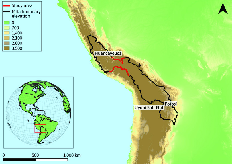
Figure 5.12 Boundaries of the mining mita (treatment group).
She discovered that villages inside the boundary, which were forced to participate in the mita system, have worse outcomes today—more than 200 years later—along a variety of dimensions. She estimates that the long-run effects of the mita system lower household consumption by around 25%, increase stunting in children by around 6 percentage points, and make it more likely for current-day residents to be subsistence farmers rather than participating in agricultural markets.
She also uncovered the mechanisms through which these effects have operated. In particular, she documents how haciendas—rural estates with an attached labour force—developed primarily outside the mita catchment (because the Spanish colonial policy restricted the formation of haciendas in mita districts to minimize the competition for scarce indigenous labour). Over time, the owners of the large rural estates outside mita districts lobbied successfully for the building of roads, which connect farmers to agricultural markets—a difference that persists today.
Exercise 5.5 Persistent effects of the mita system
Read Section 4 of Melissa Dell’s paper, which focuses on the explanations for persistent effects of the mita system. (This section contains technical details of the data used and statistical methods, which are not required to complete this exercise.) For each of these explanations, summarize why it contributed to persistent differences between communities affected by the mita system and communities that did not:
- land tenure and labour systems
- public goods provision
- labour force participation.
