Unit 8 Economic dynamics: Financial and environmental crises
8.11 A model of environmental collapse: The disappearance of Arctic sea ice
A good tool, like a power drill, has many applications. And the same is true of the tools that economists use, that is to say, models. We now adapt the model of the price dynamics curve (PDC) and tipping points from the house price example to develop the environmental dynamics curve (EDC) and the environmental tipping point arising from the effect of global warming on the extent of summer sea ice in the Arctic. We will show the process the EDC is useful for a range of environmental problems.
Positive feedback processes and the prospect of runaway climate change
Climate change is potentially a case of positive feedback and instability on a much greater scale than the housing market. We will look at the process by which the interaction of the economy and biosphere, instead of stabilizing a sustainable environment by means of negative feedbacks, can produce positive feedbacks driving the planet away from a sustainable equilibrium. The result can be a process of runaway environmental collapse.
Long before humans began to have a substantial effect on the rest of the biosphere, the natural environment was constantly changing as a result of the chemical and physical processes that make up the biosphere. Over tens of thousands of years, an ice age would give way to a period of warming in which glaciers and sea ice covers retreated towards the poles, to be followed by a new period of cold temperatures with the advance of the ice sheets into what are now temperate climates. On shorter time scales, clouds of dust sent up by massive volcanic eruptions blocked out the sun, as occurred during the ‘little ice age’ 500 years ago. (The drop in average temperature around the middle of the fifteenth century is shown in Figure 1.2b of the microeconomics volume).
Today, human economic activity is a major influence on our environment, but it is a process with its own dynamics of change. A challenge to environmental policymaking is that changes to environmental systems can set in motion runaway (positive) feedback processes so that small initial changes eventually lead to much larger effects, resulting in accelerating deterioration of the environment.
In the Amazon, for example, deforestation has already become a positive feedback process leading to ever greater portions of the once lush area being converted to dry grasslands. Deforestation due to clearing land for farming reduces rainfall. The resulting drought conditions then increase the likelihood of forest fires, which further reduce the extent of forests, setting off a vicious cycle. Past a certain level of deforestation, the process of positive feedback takes over, and will continue on its own even without further expansion of farming.
Some other examples: the historically unprecedented wildfires in Canada in 2023 released substantial amounts of carbon into the atmosphere, accelerating global warming, which in turn made massive fires more likely. Like the Amazon and the Canadian forests, many freshwater systems such as lakes and rivers are subject to vicious circles of deterioration and collapse. Another set of positive feedback processes is that rising temperatures in the warmer regions of the world lead to greater use of air conditioning in homes and public buildings, and the resulting CO2 emissions contribute to yet further warming.
Figure 8.26 describes these and some other cases of positive feedbacks threatening to destabilize our environment. What they have in common is that a warmer climate results in additional changes—in nature, or in human behaviour—that contribute to further warming.
The case of Arctic sea ice is an example of an environmental system that due to global climate change may already have shifted irreversibly away from a sustainable equilibrium. Figure 8.25 shows that for the past 50 years, the extent of the sea ice at the end of summer has been declining at an increasing rate. The satellite observations in the figure illustrate the change in the last few decades.

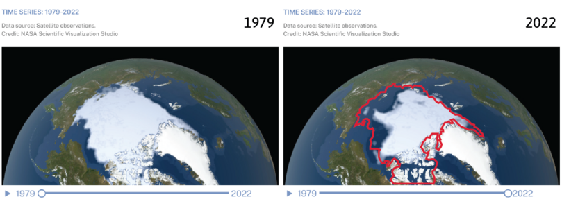
Figure 8.25 Decline of Arctic summer sea ice.
National Aeronautics and Space Administration (NASA). ‘Arctic Sea Ice Extent’.
Climate science has uncovered the mechanism that stabilized the extensive coverage of summer sea ice prior to the 1970s. By reflecting radiation, the extensive ice sheet reduces temperature and maintains the ice through the summer. But if the earth’s temperature warms sufficiently, then the negative feedbacks stabilizing the sea ice are overwhelmed and the opposite occurs. Positive feedbacks then reinforce a movement away from an equilibrium. In this case, starting from extensive sea ice, a reduction in sea ice leads to reduction of the reflection of the sun’s rays, leading to even greater reductions in sea ice, and so on.
Figure 8.26 brings together channels and feedback processes that accelerate climate change, as well as considering potential stabilizing mechanisms.
| Channels and feedbacks | Positive feedback mechanisms | Potential stabilizing mechanisms? |
|---|---|---|
| Melting polar ice caps, sea ice, Himalayan and other glaciers | Reduces reflection of sun’s rays, increasing global warming. | None, other than futuristic geoengineering, for example, spraying sea water onto the Greenland ice sheet to try to restore ice cover. |
| Melting permafrost in the Arctic tundra | Releases trapped methane, about 80 times more potent a greenhouse gas than CO2. | New plant growth in the Arctic, absorbing CO2. However, the timescale is likely to be far too slow, compared with the release of trapped methane. |
| Warming of tundra soil | Will release large amounts of buried carbon over a longer time scale. | New plant growth in the Arctic, absorbing CO2, but may be too slow. |
| Tropical rain forests and Northern boreal forests, stressed by drought; Amazon rainforests also deliberately burned to create farmland | Reverse the carbon cycle and release CO2 instead of absorbing it, for example, through the increased frequency of wildfires, triggered by lightning storms made more frequent by more volatile weather patterns caused by increased atmospheric humidity and other aspects of climate change. | Stopping human-made forest burning and attempting to reforest. Risk is that local tipping points, for example, in the Amazon or African rainforests will be reached first. |
| Human feedback | Rising temperatures increase demand for air conditioning, increasing demand for fossil fuels and CO2 release. | Rapid transition to photovoltaic power generation would mitigate the impact. |
Figure 8.26 Positive feedback processes accelerating climate change.
The figure is adapted from Table 1 in Muellbauer and Aron (2022).
We now use our model of positive feedback, lock-in, tipping points, and equilibria to better understand environmental crises. As in the case of house prices, an apparently stable situation, taken as normal for long periods, may be disrupted—resulting in changes that are both very large and difficult to reverse.
Modelling an environmental crisis
To model why we would expect to observe either extensive summer sea ice or its absence, we combine the climate science summarized above with a graphical model of the dynamic processes. You will note the similarity between Figure 8.27 and Figure 8.14 of boom and bust in a housing market. But now, instead of the house price this year and next on the axes in the figure, the horizontal axis is the extent of sea ice today (period t refers to the environment this year). The vertical axis is sea ice next year. This figure shows how the extent of sea ice today maps to the extent of sea ice tomorrow. We adapt this model to examine the movement away from the sustainable equilibrium with extensive sea ice and the process of environmental collapse, just as we did in Section 8.5 to study a house price bubble and subsequent crash.

Figure 8.27 Environmental dynamics, multiple equilibria, and the S-shaped EDC.
The 45-degree line in Figure 8.27 depicts an unchanging environment, since along that line any value of sea ice this period on the horizontal axis is the same as the next period (on the vertical axis). The S-shaped curve is the ‘environmental dynamics curve’ or EDC for short. It captures the important geological fact that holding constant other environmental influences (such as the stock of greenhouse gas emissions in the atmosphere), how much ice there is next year depends on how much ice there is this year.
To refresh your memory about the dynamics of the negative feedback process when the slope of the EDC is less than 45-degrees, go to Figure 8.13 (right panel), where the shock and adjustment process is explained using the PDC.
The EDC is S-shaped for the following reasons. First when there is little sea ice (as at the lower intersection with the 45-degree line (point B) in Figure 8.27, a small increase in sea ice in one year has very little effect on temperature, and hence on the amount of sea ice next year. So the EDC is close to being horizontal (flatter than the 45-degree line). Winter and spring surface temperatures remain high, and there is less sea ice next summer. This is a negative feedback process and a vicious circle in climate dynamics. Here we are stuck at a little-ice equilibrium.
And similarly, when there is very extensive sea ice in one year (ice extending into relatively warmer climates, the upper intersection at point G) a small decrease in sea ice will not have enough of an effect (absorbing rather than reflecting radiation) to reduce by much the extent of sea ice in the next year. So again, there is a negative feedback process and the EDC is also almost flat—a virtuous circle in climate dynamics. If either equilibria exists, it will be maintained. These negative feedbacks are summarized in Figure 8.28.

Figure 8.28 Negative feedback processes stabilize a ‘good equilibrium’ on the left, and a ‘bad equilibrium’ on the right.
If the world is at the ‘good equilibrium’ with extensive sea ice (point G) there are two things that might disrupt this:
- Shocks (movement along the EDC): occur when there is a change in the sea ice extent itself. A shock to this occurring for reasons outside the model (for example, a very hot or very cold year), would result in the extent of sea ice being greater or lesser than at point G.
- Shifts (movement of the whole EDC): occur when there is change in the process of warming occurring throughout the world for reasons other than the extent of sea ice. For example, more warming will shift the EDC downward, meaning that for some given amount of sea ice this year the amount next year will be less than before.
Both shocks and shifts are termed exogenous because their causes are external to the model. We now take up how shocks and then shifts may disrupt the good equilibrium with extensive sea ice. (The analysis parallels that of shocks and shifts to house prices.)
Shocks and the tipping point
At any point in between the two stable equilibria at G and B, from year to year the sea ice cover will either be increasing towards the virtuous equilibrium at G or disappearing towards the little-sea-ice vicious equilibrium at B. Suppose there is extensive sea ice such that the system is near point G, but for some reason—perhaps an unusually hot year, for example—the extent of sea ice is equal to E0, in Figure 8.29, that is, less than the equilibrium level at B. The EDC shows the extent of ice will be greater than E0 the following year and the arrows indicate the adjustment back to the equilibrium at point G.

Figure 8.29 Stabilization of sea ice following a shock from G to E0.
This occurs because the EDC is above the 45-degree line. When there is a lot of ice, the feedback in the direction of maintaining the ice cover is strong, and we tend to stay there even when variations in temperatures (due to seasonal or decadal variation in ocean currents) cause temporary warming and temporary reductions in sea ice. The extent of the ice means that the system ‘rebounds’ towards the high equilibrium as it did in Figure 8.25 prior to 1970.
This is an example of a negative feedback process in which an initial shock which moves the system away from the equilibrium point is dampened so that the subsequent changes are in the opposite direction, counteracting the initial shock. If there is a small negative shock away from point G—a slight reduction in the amount of ice—then in later periods if there are no further shocks, the initial extent of the ice will be restored. But what happens if the shock is too large?
You can refer back to the model of house price dynamics in Figure 8.14 for the adjustment processes around a stable and an unstable equilibrium.
In addition to the two stable equilibria at B and G in Figure 8.29, there is also an unstable equilibrium at point T (the tipping point). If for some reason—a chance succession of unusually hot years, for example—the extent of sea ice is reduced below the level at the tipping point, the process works in the opposite direction.
The process amplifies the initial shock (reduced sea ice) rather than dampening it. At that point, the positive feedback reduces the ice cover, bringing the system to the little-Arctic-summer-ice state. The capacity of the system to recover would have been pushed beyond its limits. Environmental scientists are increasingly pointing to the existence and importance of tipping points in environmental systems, which represent a point which, if passed, sets in motion a process leading to abrupt and hard-to-reverse destruction of an environmental resource.
Shifts in the EDC due to climate change
What is the role of climate change in all this? To analyse this, we need to explain why the S-shaped environmental dynamics curve can shift down. If it shifts far enough, the system will not stabilize around the extensive-summer-ice equilibrium at G.
To understand these effects, consider Figure 8.30. A warmer climate means that for any amount of sea ice this year, the amount that will be there next year is less. G is no longer an equilibrium. This is not a movement along the horizontal axis. Rather it fixes a point vertically below point G on a new EDC, labelled EDC′, shown in the left panel.

Figure 8.30 Climate change causes the EDC to shift down.
As a result of the downward shift of the EDC, less ice forms in the winter and the whole system is more vulnerable to the increase in temperature and open surface area in the summer.
A warming climate
Starting from the high equilibrium, the downward shift in the EDC brings the new virtuous equilibrium G′ and the tipping point T′ closer together and widens the ‘danger zone’ of environmental collapse.
In Figure 8.30, the shift down in the EDC means that it will take a smaller shock—perhaps just one unusually hot year—to push the system past the tipping point into the region where positive feedbacks take over, driving the system to the little-summer-ice equilibrium. And if a downward shift in the EDC is large enough, it will change the system such that the equilibrium with extensive summer sea ice disappears, as shown in the right panel of Figure 8.30.
Combining the model and the available evidence, the change from the Arctic with extensive-summer-ice to the Arctic with little-summer-ice equilibria appears to be underway. It appears to be much slower than the deforestation of the Amazon, but it is happening. Scientists are unsure how reversible this loss of the Arctic summer ice is even if we reverse global warming. We may have crossed a point of no return. The lack of Arctic sea ice—if that is what is in store—will add to the already powerful forces creating a warmer climate.
Exercise 8.9 Environmental tipping points
The Regime Shifts DataBase documents different types of regime shifts (another word for tipping point) that we have evidence for in human-dominated ecological systems. Choose one from the database and describe the situation in your own words, including the types of equilibria and their characteristics, and how the system transitions from one equilibrium to another. Draw diagrams similar to Figure 8.10 and Figure 8.30 to represent it, and explain the feedback loops that are involved.
