Unit 4 Inflation and unemployment

4.4 Inflation, unemployment, and conflicting claims on output

When inflation is mentioned, the word that often springs to mind is ‘money’. This makes some sense because when prices are rising, (nominal) wages measured in dollars or euros can purchase fewer goods and services. ‘Inflation means that a given amount of money buys less.’ This describes one consequence of inflation, but not why it happens. What drives the process of inflation is not ‘money’ but the dynamics of wage setting and price setting, as described in Unit 1. In this and the following section, we directly connect the WS–PS model with why wages and prices across the economy as a whole change, and therefore with inflation. When we studied the WS–PS model before, attention was on the outcomes for real wages and unemployment; now, it is also on the outcome for inflation.

Conflicting claims

structural unemployment

The level of unemployment where the supply side of the economy is in equilibrium. In the WS–PS model, it is the unemployment level at which the price-setting real wage equals the wage-setting real wage. See also: WS–PS model, Nash equilibrium, supply side.

At the heart of the process of inflation is the conflict of interest between workers and owners over the share of output per worker that each group gets—the wage share and the profit share. In the WS–PS model, the conflict is resolved at a particular level of employment on the horizontal axis where the WS curve and the PS curve intersect. The unemployment rate associated with this intersection is the economy’s structural unemployment rate. To the right of the intersection, where employment is higher, unemployment is lower than the structural rate and wages and prices tend to rise; and on the left, where unemployment is higher, they tend to fall (read Section 1.8). This provides the intuition behind the Phillips curve, which relates the unemployment rate to the rate of inflation.

To develop your intuition, think as before of an economy composed of many identical firms (each of which is owned by a single individual) and their employees, who are also the consumers of the goods produced by the firms. To keep track of what is happening in the firms, we assume as in Unit 1 that wages are set by the human resources (HR) department and prices are set by the marketing department.

According to the wage-setting model from Section 1.6, the HR department in each firm sets the nominal wage for its workers at the level required to recruit sufficient workers and motivate them to work hard—the ‘no-shirking’ wage. When divided by the price level in the economy to get the wage in terms of what can be purchased, this is the real wage on the WS curve at the prevailing unemployment rate in the economy.

Meanwhile, according to the price-setting model from Section 1.7, the marketing department in each firm sets its price as a markup over its marginal cost to maximize its profits, given the degree of competition in the markets in which it sells (recall that profit maximization occurs where the markup is inversely proportional to the price elasticity of demand, which is affected by the degree of competition). The outcome of the price-setting process across the economy can be expressed as a ratio of the nominal wage to the price set. This is the price-setting real wage.

supply-side equilibrium

The economy is in supply-side equilibrium when the markets involved in the production of output are in equilibrium. In the WS–PS model it is the labour market equilibrium; that is, where the price-setting real wage equals the wage-setting real wage.

goods market equilibrium

A goods market is in equilibrium when the supply of goods is equal to the demand. In the multiplier model, aggregate demand for goods and services, AD, depends on income, Y, and income is equal to the output that firms supply. Goods market equilibrium is at the value of Y where aggregate demand is equal to output: AD = Y.

If, having set their wages and prices at the same levels as in the previous year, enough workers are hired and profits are maximized, then wage and price setters are satisfied. There is no reason for either prices or wages to be changed and at this unemployment rate, both wage and price inflation are zero. This is the rate of un­employment where the wage-setting and price-setting curves intersect, that is, the Nash equilibrium from Unit 1, which we call the supply-side equilibrium for short.

At the supply-side equilibrium in Figure 4.5 at point A, the real wage on the WS curve is equal to \((1 - \sigma)\lambda\) on the PS curve. The real profit per worker is equal to \(\sigma\lambda\). They sum to \(\lambda\), that is, to output per worker. Another way of saying this is that the claims of workers and of owners to output per worker are compatible at the equilibrium unemployment rate.

Fullscreen

https://www.core-econ.org/macroeconomics/04-inflation-and-employment-04-inflation-unemployment-conflicting-claims.html#figure-4-5

Figure 4.5 Supply-side equilibrium: claims on output per worker by workers and owners are compatible.

But when the economy is not in supply-side equilibrium—in particular when unemployment is below the equilibrium level—inflation occurs. To the right of A in Figure 4.5, the wage on the WS curve is above that on the PS curve. If, at the lower unemployment rate, workers are to get the real wage on the WS curve, which is now above the PS curve, then real profit per worker will be squeezed below \(\sigma\lambda\).

At lower unemployment, the HR departments of firms will increase nominal wages. This will increase firms’ costs, and marketing departments will immediately pass on the cost increase in higher prices as they aim to restore the profit share to \(\sigma\). Both nominal wages and prices will rise. Rising wages and prices are a symptom of the conflicting claims of the two groups—workers and owners—on output per worker.

Figure 4.6 shows the causal chain from lower unemployment to inflation. We work through causal change in detail in the next section.

Fullscreen

https://www.core-econ.org/macroeconomics/04-inflation-and-employment-04-inflation-unemployment-conflicting-claims.html#figure-4-6

Figure 4.6 Causal chain from lower unemployment to higher inflation.

And remember that, in this model, firms set their prices immediately after nominal wages are set, returning the real wage to the PS curve.

As long as unemployment remains below equilibrium, \(\text{WS} > \text{PS}\) and the process of rising wages and prices continues. Lower unemployment is associated with a higher rate of wage and price inflation.

Question 4.3 Choose the correct answer(s)

Based on the information shown in the diagram, read the following statements and choose the correct option(s).

Fullscreen

• If the real wage was equal to the level on the WS shown by point B, the markup is too high.
• Point B illustrates workers’ better alternative opportunities in the labour market at low unemployment.
• The gap between the price-setting real wage and the wage demanded on the wage-setting curve pushes prices upwards.
• The conflicting claims on output per worker must lead to an increase in the real wage when employment is higher than at point A (for example, at point B).

• The real wage at point B is above the price-setting curve, which means it is higher than is consistent with a firm’s profit-maximizing markup. If the real wage is too high, it means the markup is too low.
• At lower levels of unemployment, workers can easily find other jobs in the labour market and are offered higher nominal wages by HR.
• \(\text{WS} > \text{PS}\) produces higher nominal wages, which are passed on in higher prices.
• Both nominal wages (W) and prices (P) increase by the same percentage (to restore the profit share back to its original level), so the real wage remains the same (on the PS curve). Firms have the power to set the real wage workers get.

Bringing the supply and demand sides together: Aggregate demand, unemployment, and inflation

In Unit 3, we used the multiplier model to explain how the economy fluctuates between upswings and downswings as a consequence of shifts in aggregate demand. Combining this with the supply-side model, we can now show how aggregate demand, unemployment, and inflation are linked together.

production function

A production function is a graphical or mathematical description of the relationship between the quantities of the inputs to a production process and the amount of output produced.

wage inflation

An increase in the level of the nominal wage, usually measured as the percentage increase over one year. See also: nominal wage.

Phillips curve

An inverse relationship between the rate of inflation and the rate of unemployment. It is named after Bill Phillips, who observed the relationship empirically, but it can also be derived from a theoretical model of wage and price setting.

When output rises because of a rise in demand, unemployment falls. The data in Figure 3.8 shows that unemployment goes down in booms and up in recessions. And it follows directly from the assumptions in our supply-side model: as explained in Section 1.5, labour is the only input to production, and output per worker (labour productivity) is a constant, \(\lambda\). In other words, the production function—the relationship between output and the inputs used to produce it—is:

This production function means that in our model, output and employment are directly proportional to each other; when output rises, employment rises in proportion, and unemployment falls. The resulting causal chain is shown in Figure 4.7.

Fullscreen

https://www.core-econ.org/macroeconomics/04-inflation-and-employment-04-inflation-unemployment-conflicting-claims.html#figure-4-7

Figure 4.7 Adding output to the causal chain from higher aggregate demand to lower unemployment and higher inflation.

The Phillips curve: Unemployment and inflation

The notion built into our model that lower unemployment may result in inflation first came to light when William (Bill) Phillips, the economist, examined the data. He published a scatterplot of annual wage inflation and unemployment in the British economy over a period of more than 50 years. This is shown in Figure 4.8. Note that the unemployment rate decreases to the right along the horizontal axis to match the format of the model, where we derive the Phillips curve. An unemployment rate of around 7% was associated with constant wages (zero-wage inflation). Rising wages were observed on many more occasions than falling wages.

Fullscreen

https://www.core-econ.org/macroeconomics/04-inflation-and-employment-04-inflation-unemployment-conflicting-claims.html#figure-4-8

Figure 4.8 Phillips’s original data and curve: wage inflation and unemployment (1861–1913). Note the inverted scale on the horizontal axis with unemployment falling from left to right. His method for estimating a best-fit curve was different from the methods used now. To view a different visualization of this data with unemployment rising along the horizontal axis, go to OWiD.

View interactive graph View static graph

Great economists Bill Phillips

A. W. (‘Bill’) Phillips (1914–1975) was an unusually colourful character for a world-renowned economist. Raised in New Zealand, Phillips spent time as a croco­dile hunter, a movie director, and a prisoner of war in Indonesia during the Second World War, before finally becoming a professor at the London School of Economics.

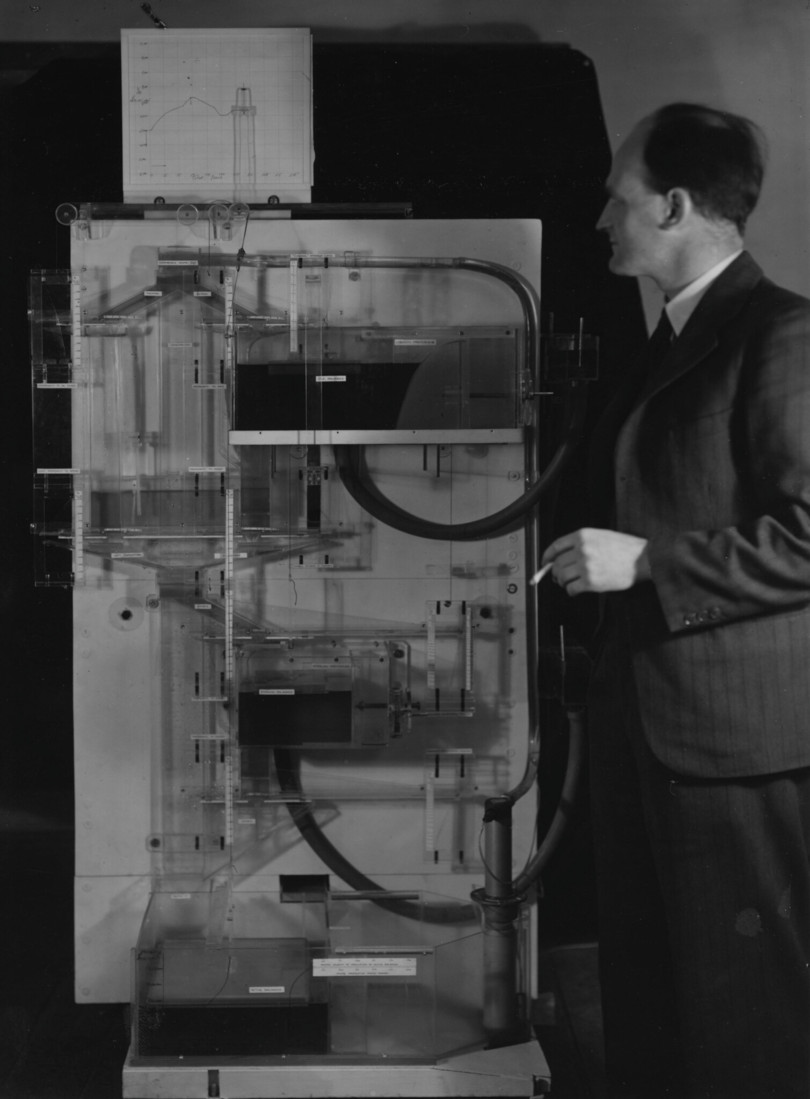
This is Arthur Phillips with the MONIAC machine he built.

Phillips had engineering know-how and, while studying sociology in London in 1949, he built a hydraulic machine to model the British economy. The Monetary National Income Analogue Computer (MONIAC) used transparent pipes and coloured water to bring economists’ equations to life. MONIAC had tanks for each of the components of domestic GDP, such as investment, consumption, and government expenditures. Imports and exports were shown by water being added or drained from the model. The machine could be used to model the effect on the economy of shocks to different variables, such as tax rates and government spending, which would set in motion flows between the tanks. Working versions of the machine can still be found in the London Science Museum and universities around the world.³

In a 1958 paper, Phillips made another major contribution to the study of economics. By drawing a scatterplot of the data for the rates of unemployment and inflation in the British economy between 1861 and 1913, he found that low rates of unemployment were associated with high rates of inflation, and high unemployment with low inflation. The relationship has since been referred to as the Phillips curve.