Unit 5 Macroeconomic policy: Inflation and unemployment
5.11 Application: Inflation and the monetary policy response to the Russia–Ukraine war
In this section, we use an interactive tool (CORE Econ’s inflation tool) to explore the problem facing central banks when inflation increased rapidly in the aftermath of the pandemic. The macroeconomic modelling you have studied in this unit provides essential background to the policy simulation in this tool.
The tool has four parts. The first two parts of the interactive tool reinforce what has been covered in the unit and apply it to the recent resurgence of inflation and the problems it has caused for central banks. As an extension to the activities in this section, you can try parts 3 and 4, which go beyond the modelling covered in this unit by introducing more detail about the central bank’s preferences.
Exercise 5.7 Introduction to the inflation tool: A supply shock
Open the inflation tool. The opening page will look like Figure 5.15. Read the first section and the ‘Supply shock’ section.
Figure 5.15 Opening page of CORE Econ’s inflation tool.
Figure 2 of the inflation tool shows a rise in inflation from 2% to 5% due to an oil price shock in period 4. Suppose there is no policy response by the central bank to this shock.
- Draw a diagram like Figure 5.13 (top panel) to illustrate the initial effects of the oil price shock.
- Draw a diagram like Figure 4.16 (Unit 4) to show the path of inflation in periods 4 to 10. Your diagram should look like the stepwise version of Figure 3 in the inflation tool.
Exercise 5.8 The oil shock and the central bank’s policy choice
As discussed in Section 5.10, the central bank will want to prevent the scenario shown in Figure 3 of the inflation tool from occurring.
- In the inflation tool, go to the box titled ‘Question: Monetary policy reaction to an inflation shock’ (shown in the first panel of Figure 5.16) and use the slider to choose the real interest rate for the next period to try to stabilize inflation. Click ‘Submit’ to reveal the outcomes of your choice, with an explanation (the second panel of Figure 5.16). To try another interest rate, click ‘Reset’.
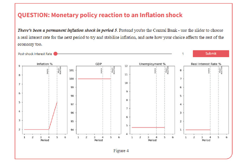
Figure 5.16a An oil shock hits the economy.
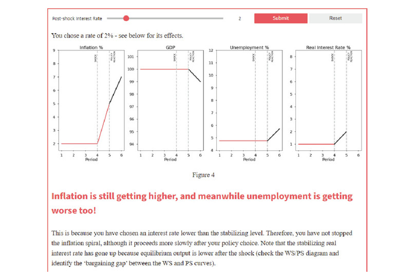
Figure 5.16b Choose the central bank’s interest rate response and observe the economic outcomes.
You can verify that by choosing the appropriate interest rate, the central bank manages to bring inflation back to target. But could the central bank do even better, in terms of inflation?
- Discuss whether the central bank could avoid the increase of inflation in the shock period. Why or why not?
- Choose different values for the interest rate and comment on how sensitive GDP is to the chosen interest rate and the slope of the Phillips curve. (Hint: both slopes are integers.)
- There is evidence that the Phillips curve has flattened during the last decades (for example, as shown in Prospects for inflation: sneezes and breezes). Discuss how the flattening of the Phillips curve may affect the cost of bringing inflation down after the supply shock.
Part 2 of the inflation tool gives you the opportunity to experiment with different central bank approaches to the inflation problem it faces. One approach has similarities with the UK’s use of tight monetary policy in the 1980s by the Thatcher government. A rapid increase in unemployment is accepted in exchange for a steep fall in inflation (Figure 5.17).
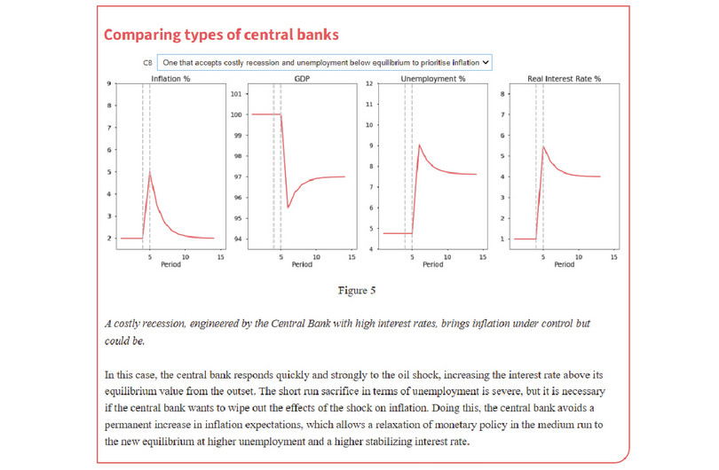
Figure 5.17 Example of the choice of policy by the central bank to respond to the increase in inflation.
Exercise 5.9 Active policy scenarios to address inflation and unemployment
Read this excerpt of a 2022 speech by Jerome Powell, chairman of the US Federal Reserve, then answer the following questions.
‘Reducing inflation is likely to require a sustained period of below-trend growth. Moreover, there will very likely be some softening of labor market conditions. While higher interest rates, slower growth, and softer labor market conditions will bring down inflation, they will also bring some pain to households and businesses. These are the unfortunate costs of reducing inflation. But a failure to restore price stability would mean far greater pain.[…] During the 1970s, as inflation climbed, the anticipation of high inflation became entrenched in the economic decision making of households and businesses. The more inflation rose, the more people came to expect it to remain high, and they built that belief into wage and pricing decisions. […] History shows that the employment costs of bringing down inflation are likely to increase with delay, as high inflation becomes more entrenched in wage and price setting. The successful Volcker disinflation in the early 1980s followed multiple failed attempts to lower inflation over the previous 15 years. A lengthy period of very restrictive monetary policy was ultimately needed to stem the high inflation and start the process of getting inflation down to the low and stable levels that were the norm until the spring of last year. Our aim is to avoid that outcome by acting with resolve now.’
- Explain what you think Jerome Powell means by the ‘softening of labor market conditions’.
- Explain which of the two active policy scenarios (‘central bank that slowly accepts change to unemployment’ and ‘central bank that accepts costly recession and unemployment below equilibrium to prioritize inflation’) better fits the 1970s experience described by Powell.
- Which of the two active policy scenarios better fits Powell’s intentions in 2022? Why?
Consider scenario 3 in the ‘Comparing types of central banks’ simulation, where the central bank quickly reacts to the shock. In this scenario, the interest rate and the unemployment rate peak to 5.5% and 9%, respectively. Now consider scenario 2 (the central bank slowly accepts changes to unemployment) and suppose that in period 15, the central bank resolves to tighten monetary policy in order to bring inflation back to the target.
- Use the information in the ‘Comparing types of central banks’ simulation and Powell’s speech to explain whether: i) monetary policy in scenario 2 should be tighter or less tight compared to scenario 3, and ii) unemployment would be higher or lower compared to scenario 3.
Question 5.9 Choose the correct answer(s)
Read the following statements about the inflation shock in Figure 2 of the inflation tool and choose the correct option(s).
- The term inflation shock is used to refer to an exogenous shift in the Phillips curve.
- The opposite is true: the central bank needs to increase the interest rate immediately to decrease output below equilibrium.
- Inflation decreases if the nominal interest rate is above the stabilizing interest rate. It could be that the interest rate is increasing, but it is still below the stabilizing interest rate. Then inflation increases.
- The central bank could stabilize inflation but unemployment would rise, or tolerate higher inflation while maintaining the level of employment.
Question 5.10 Choose the correct answer(s)
Based on the information in Figure 5 of the inflation tool, read the following statements and choose the correct option(s).
- If the central bank does not change the interest rate, inflation rises period by period. It will eventually have to change its policy and accept costly recession and unemployment above equilibrium to reduce inflation.
- The policy succeeds in stabilizing inflation at the cost of higher unemployment, but at a higher inflation rate than the central bank’s target of 2%. The answer would be correct only if the central bank changed its inflation target to 4%.
- Although costly, that is the only way to bring inflation down to its target.
- If the central bank does not react quickly and strongly to the oil shock, inflation expectations could increase permanently.
