
Unit 5 The rules of the game: Who gets what and why
5.8 Case 3: Bargaining in a democracy
In the final situation, Case 3, Bruno owns the farm and Angela is Bruno’s employee. As in Case 2, Bruno’s property rights and Angela’s right not to agree to a contract are protected by law. But there is an important difference, which leads to a different employment contract from the one in Case 2.
In Case 3, Angela is a voter and is free to seek change in the legal institutional arrangements, together with other farmworkers. She has democratic political rights. Case 3 therefore represents a common economic interaction in modern capitalist economies with a democratic form of government. Angela’s vote, and that of other workers, can bring about legal changes in the rules of the game by influencing the government.
In this section, we describe the legal changes they achieve, and how these affect the contract that Bruno offers Angela. The following section will consider what happens when, rather than simply accepting a take-it-or-leave it offer, she has scope to negotiate further changes with Bruno.
Angela’s and Bruno’s actions and the outcomes when Angela votes for specific worker rights
Suppose that Angela and others who work on neighbouring farms lobby the government to improve their conditions. They want working hours for farm labourers restricted to four and a half hours per day. They also want to get at least the same amount of grain as under the voluntary take-it-or-leave-it contract agreement in Case 2, which was 23 bushels. Angela, and other workers, will vote for the political party that agrees to implement their demands. They use their ability as voters to make legislative demands on the government, thereby influencing their employment contracts.
The government agrees to the demands of the farm labourers, hoping to secure their vote in subsequent elections. So Bruno is constrained to offer a contract with working hours between zero and four and a half hours per day. He must also ensure that Angela gets at least 23 bushels of grain. Work through Figure 5.16 to figure out his choice.
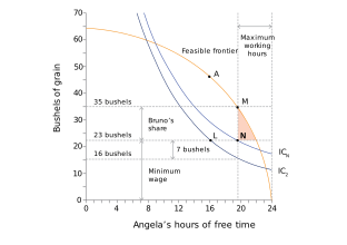
Figure 5.16 The effect of a law setting maximum working hours and minimum pay.
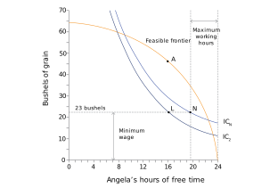
The new law improves Angela’s reservation position
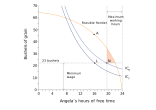
The new law limits Bruno’s options
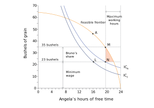
The contract Bruno will offer
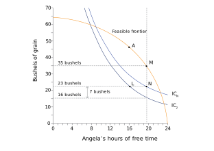
Angela will produce less grain and get higher utility
Under the new legal constraints, the best Bruno can do is to offer Angela the minimum daily wage (23 bushels) for the maximum number of hours (4.5). To maximize his amount of grain, he keeps the wage as low as possible. And if he gave Angela more free time, less grain would be produced; he would still have to pay her at least 23 bushels, leaving less for himself.
He offers Angela contract N. If Angela accepts, she produces 35 bushels of grain (point M). After paying her wage of 23 bushels, he obtains a rent of 12 bushels. Angela gets her new reservation utility, so her rent is zero. The total surplus (the sum of Bruno’s and Angela’s rents) is 12 bushels.
Although less grain is produced than in Case 2, and Angela still gets no rent, she is undoubtedly better off as a result of the new law. At allocation N, her wage is the same as before, but she has more free time, so we know that her utility is higher. And we can measure the increase in utility: the new law has raised her reservation indifference curve by seven bushels from IC2 to ICN, so her utility has risen by the equivalent of seven bushels of grain.
Figure 5.17 summarizes the allocation. But, as the next section discusses, this may not be the outcome. Both Angela and Bruno can do better.
| Angela’s hours of free time | 19.5 | |
| Angela’s bushels of grain | 23 | |
| Bruno’s bushels of grain | 12 | |
| Angela’s economic rent (bushels) | 0 | She is on ICN, her new reservation indifference curve |
| Bruno’s economic rent (bushels) | 12 | His best alternative is 0 (if Angela refuses to work for him) |
Figure 5.17 The allocation under contract N, satisfying the new minimum wage and maximum hours law.
Question 5.5 Choose the correct answer(s)
Figure 5.16 shows the outcomes before and after the introduction of a new law that limits Angela’s maximum working hours to four and a half hours a day and requires that she receive at least 23 bushels of grain. Contract N is Bruno’s first offer to Angela. Based on this information, read the following statements and choose the correct option(s).
- It is not a Pareto improvement, because Bruno is worse off (gets less grain) at N than at L.
- Contract N is on a higher indifference curve than L.
- At N, Angela is on her new reservation indifference curve and therefore does not receive any economic rent. Bruno’s reservation option is to receive nothing, so the grain he receives at N is an economic rent for him.
- The law has increased Angela’s structural power and reduced Bruno’s, because Angela can now walk away from L. Now her new reservation utility is contract N.
In this ‘How economists learn from facts’ feature, economist Gabriela Deschamps discusses research on how a change in the law to allow unilateral divorce in some states in the US affected women’s reservation options; economists were able to measure this by using data on domestic violence.
How economists learn from facts Divorce law and domestic violence
We have modelled employment relationships as a game between employer and employee, in which the outcome depends on their bargaining power (shaped by the rules of the game) and their structural power (the value of walking away). Economists have used a similar approach to model relationships within the household. Couples can share the benefits from their relationship in different ways. When they decide how they will each spend time on childcare, household work, and employment, and what to spend money on, the resulting benefits to each party may likewise depend on their bargaining and structural power: how they make decisions, and what happens if the relationship breaks down. In the context of the household, both dimensions of power are influenced by social norms and by the legal framework governing individual behaviour, gender rights, property rights, and divorce or separation.
We will focus on one of these laws—divorce law—because it bears directly on the reservation option: it sets the terms on which a woman can legally end the marriage. Imagine a regime in which a woman can only divorce if her husband agrees. How good is her reservation option? Very poor. She can physically leave him, but without his consent she cannot legally end the marriage, cannot remarry, and cannot claim any share of the assets the couple built up. Her situation parallels Angela’s in Case 1 (forced labour): her reservation option is so poor that her partner can extract almost anything from the relationship.
Now imagine the rules change, and she can end the marriage without her husband’s consent. This is called unilateral divorce. Those who gain most from this change are the women with the strongest reasons to exit. Violent marriages are one obvious case. By giving women a credible way out, the reform has two possible effects on these marriages. First, some violent marriages may end, as women leave abusive partners. Second, even in marriages that continue, the threat of exit may deter abusive behaviour. Either way, the prediction is the same: fewer women experiencing violence from their partners.
Economists Betsey Stevenson and Justin Wolfers tested this prediction using a natural experiment from the United States. Until the late 1960s, US divorce law required either both spouses to consent or one to prove the other guilty of misconduct (such as adultery, desertion, or documented cruelty) in court—a high bar that often required witnesses or physical evidence. In 1969, California became the first state to adopt unilateral divorce. Through the 1970s and 1980s, most other US states followed.
How could they tell whether the reform actually reduced violence? They couldn’t simply look at what happened in reforming states before and after the reform, because lots of other things were changing in American marriages over these decades. Attitudes were shifting, more women were working, and the economy went through ups and downs. Any of these could have reduced violence on its own.
The trick is to also look at the states that did not reform. Before the reforms, violence had been evolving similarly in the two groups of states. There is little reason to think it would have evolved differently in one group than the other in the absence of the law. Both were exposed to the same shifting attitudes, the same labour market changes, and the same economy. The only systematic difference between them was that one group changed its divorce law and the other did not. So whatever change in violence happened in non-reforming states is roughly what would have happened in the reforming states anyway. If violence fell much more in reforming states than in non-reforming states, the extra fall can be attributed to the change in the law. Figure 5.17b illustrates the comparison between reforming and non-reforming states. This way of comparing two groups—one exposed to a change, one not—before and after the change is called difference-in-differences. It is one of the most widely used techniques in empirical economics.
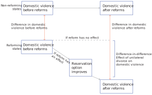
Figure 5.17b Estimating the causal effect of unilateral divorce on domestic violence.
Stevenson and Wolfers applied this approach to several different outcomes, drawing on different datasets. They looked at self-reported domestic violence from a national survey of women, at female suicide rates, and at the rate of women murdered by their partners. Each measure has its limitations—survey responses depend on what women are willing to report; suicide and homicide are extreme outcomes that capture only the worst cases—so finding the same pattern across all three is more convincing than any single measure on its own.
The three measures pointed in the same direction. Take domestic violence, for example. In non-reforming states it rose by around 2.5 percentage points, and the assumption is that reforming states would have risen by the same amount had the law not changed. Instead, violence in reforming states fell by 1.7 percentage points. The gap between the two (around 4 percentage points) is the effect attributed to the reform: a fall of around 30%. On the same basis, female suicide fell by around 10% over the two decades following the reform. Partner homicides of women also fell in reforming states, though some of the decline appeared to begin before the law changed, which makes the homicide result harder to attribute cleanly to the reform. Although our discussion has taken the woman’s perspective, the survey recorded violence by and against both spouses, and the reform reduced domestic violence by roughly the same amount for husbands and wives.1 2
Exercise 5.6 Analysing difference-in-differences
- Suppose a country adopts unilateral divorce, but social stigma is so strong that divorced women face severe consequences. Would you expect violence inside marriages to fall after the reform? Why or why not?
- In your own words, explain the difference-in-differences method. Why is it not enough to compare violence in reforming states before and after the law changed?
- For each of the three measures Stevenson and Wolfers used, give one strength and one weakness. Why is finding the same pattern across all three more convincing than finding it in any one of them?
-
Betsey Stevenson and Justin Wolfers. 2006. ‘Bargaining in the Shadow of the Law: Divorce Laws and Family Distress’. Quarterly Journal of Economics 121 (1): pp. 267–288. ↩
-
Suicide data can be accessed through CDC Wonder. ↩
