Unit 9 Uneven development on a global scale
9.12 Planetary limits and sustainable growth
In this section, we shall learn that the growth rates of per capita incomes in both rich countries since the early 1800s and in poorer countries during the recent period of catch-up growth have one key attribute in common. Global growth has, so far, required continuous growth of carbon emissions. But there is clear-cut scientific evidence that carbon-intensive growth is not sustainable on a planetary scale. So we ask: Can the living standards of the world’s poor continue to improve without replicating this carbon-intensive growth process?
Capitalism, carbon, and two centuries of economic growth
While a technology for carbon capture and storage exists, it is still only used on a trial basis. It is not economical even for large-scale emitters like power stations, let alone in dealing with the smaller-scale emissions from vehicles and home heating systems.
As explained in Section 2.11 of the microeconomics volume, the hockey stick growth of the Industrial Revolution was made possible by the combination of capitalist institutions and carbon-based technologies. Over the last 200 years, fossil fuels—oil, coal, and gas—have been an essential input to the production process, and since the mid-twentieth century have enabled very significant catch-up growth in the poorer countries of the world. And it is currently effectively impossible to burn fossil fuels without emitting carbon dioxide as a byproduct.
As a result, no country in the world produces output and consumption for its citizens today without also emitting carbon. Figure 9.28a shows clearly that the higher a country’s standard of living (as measured by GDP per capita on the horizontal axis) the more carbon dioxide it emits. The chart shows ‘consumption-based’ CO2 emissions for 2022, which take into account the carbon emissions produced by the goods a country imports.
To observe how the relationship between carbon emissions and living standards has changed since 1750, use the time lapse feature of Figure 9.28b. If you select only the United Kingdom, for example, you can watch the carbon emissions per capita rising with GDP per capita and then falling.

Figure 9.28a The association between GDP per capita and CO2 emissions, 2022.
R. M. Andrew, and G. P. Peters. 2024. The Global Carbon Project’s Fossil CO2 Emissions Dataset. World Bank Group. 2025. World Development Indicators.
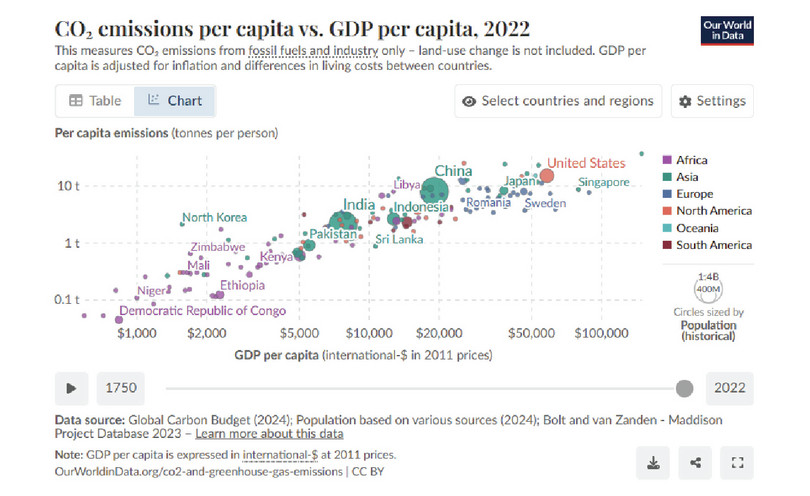
Figure 9.28b The association between GDP per capita and consumption-based CO2 emissions, 1750–2022.
Our World in Data. 2022. CO2 emissions per capita vs. GDP per capita.; Jutta Bolt and Jan Luiten van Zanden. 2024. ‘Maddison-Style Estimates of the Evolution of the World Economy: A New 2023 Update’. Journal of Economic Surveys: pp. 1–41.
The authoritative source for research and data about climate change is the Intergovernmental Panel on Climate Change.
The overwhelming majority of scientists now agree that carbon emissions, and the resulting build-up in atmospheric carbon dioxide, are the primary cause of climate change—and that the need to prevent further climate change is urgent. The 2015 Paris Agreement recognized that to avert the worst impacts of climate change, the global temperature increase must be limited to 1.5°C above pre-industrial levels. Climate researchers estimate how much more CO2 in total can be emitted in order to keep global temperature in check. Current policies as of 2023,1 have the world on course to emit more than is consistent with achieving 1.5°C; we are currently on course for warming of around 2.5°C.
Can we raise living standards and address global poverty without emitting CO2?
Sustainable economic growth
- sustainable economic growth, sustainable growth
- Growth in aggregate income (GDP) is sustainable if it occurs without reducing the capital stock or environmental resources that are needed to produce future income.
The term sustainable economic growth is based on the idea (introduced in Section 9.2 of the microeconomics volume) that what we count as income is the maximum we could consume without borrowing or otherwise reducing the value of our wealth. A family’s consumption is not sustainable if it is based on them selling their car, their house, and the other assets that make up their wealth.
Extension 1.2 of the microeconomics volume explains that the same can be said for a nation: the true (meaning sustainable) measure of a country’s income takes account of the need to replace the capital goods that are used up (worn out) in the production process. We do this in the national income accounts by subtracting depreciation of the capital stock from GDP to get net national product. Unit 1 of the microeconomics volume also explains that even net national product is not a measure of sustainable income because it omits the using up of natural resources in the process of producing goods and services. We showed, for example, that the measured economic growth of Indonesia would be substantially lower if we subtracted the used-up oil and forest resources that were part of the growth process there.
- degrowth
- The proponents of degrowth argue that production and consumption in richer countries should be reduced and redistributed to poorer countries, to protect the planet and distribute resources more fairly.
- green growth
- Growth in GDP would be ‘green’ if output were produced using technologies based on renewable environmental resources; in particular renewable energy rather than fossil fuels.
Sustainable growth is therefore the increase in output minus not only the amount of used-up conventional capital goods (depreciation of machinery, for example), but also the amount of used-up natural resources (sometimes termed natural capital). There are two strategies that have been suggested for addressing the fact that ‘capitalism + carbon’ is no longer a recipe for sustainable growth: degrowth and green growth, which we explore in the next two subsections.
Degrowth as a solution to carbon emissions?
For a helpful summary and discussion of both degrowth and green growth proposals, read Lenaerts et al. 2021.
The degrowth movement provides a broad critique of global capitalism, and in particular its focus on GDP growth. Proponents argue that per capita GDP is a very poor measure of living standards, which ignores the social and environmental values that matter for human wellbeing and the danger of ecological collapse. They propose—among other policies and recommendations—a ‘democratically led, redistributive downscaling of production and consumption in industrialized countries’.
Addressing the problem of climate change is not the only objective of the degrowth movement. Nevertheless, we can answer one of its central questions: Would a reduction in output (negative GDP growth), particularly in high-income economies, help us to address it? Figure 9.28a might suggest that if the countries on the right-hand side were to lower their GDP, global carbon emissions would fall—at least if their reduction in output were sufficient to offset any increase in poorer countries. In this case, a fall in global GDP (degrowth) would occur together with some fall in global carbon emissions.
But even if we set aside the political barriers to the reduction in GDP in the richer countries, it is clear that a simple prescription to produce and consume less, without any other changes to what we consume or how we produce it, could not in itself resolve the problem of climate change. If global GDP were lower, resulting in a proportional reduction in carbon emissions, we would not be on a path to net zero emissions. Even negative GDP growth would not be sustainable if it still resulted in catastrophic climate change.
Is green growth a solution to carbon emissions?
While Figure 9.28a shows that current production technologies remain highly reliant on fossil fuels and hence on carbon emissions, closer analysis suggests some grounds for optimism. Countries are not all producing and consuming in the same way. Among countries at the same income level, some have a much higher carbon footprint than others, by a factor of 10 or more.
This suggests that changes in the way we produce our income—new technologies—rather than simply producing less with the same technology, may provide a feasible route to emissions reduction and sustainable growth. Figure 9.29 shows that, to some extent at least, such changes have been happening. Strikingly, global CO2 emissions per capita have remained relatively flat since the oil price shocks in the early 1970s provided strong incentives to reduce reliance on oil, while GDP per capita has continued to grow. The world as a whole has got richer, in GDP per capita terms, without increasing per capita emissions.

Figure 9.29 Change in per capita CO2 emissions and GDP, 1950–2023.
R. M. Andrew, and G. P. Peters. 2024. The Global Carbon Project’s Fossil CO2 Emissions Dataset. World Bank Group. 2025. World Development Indicators.; Jutta Bolt and Jan Luiten van Zanden. 2024. ‘Maddison-Style Estimates of the Evolution of the World Economy: A New 2023 Update’. Journal of Economic Surveys: pp. 1–41.
How can this evidence be reconciled with Figure 9.28a, which shows a close relationship between CO2 emissions and GDP across countries in 2022? The answer is that as individual countries have adopted less carbon-intensive production methods, the relationship between CO2 emissions and GDP across countries has shifted to the right. The interactive version, Figure 9.28b, shows how it has moved continuously to the right since 1970, as many countries have increased income without much change in emissions.
- decoupling
- In most countries, GDP growth has been accompanied by rising carbon emissions. Some countries have recently experienced growth in GDP while reducing carbon emissions; this is referred to as ‘decoupling’.
The apparent break in the link between carbon emissions and GDP growth, known as decoupling, has occurred in the high-income countries, especially since the 1990 Kyoto conference (although world per capita emissions have risen since then). But there remain big differences between otherwise similar countries. Since 1990, consumption-based CO2 emissions per capita have fallen by 39% in the UK and an average of 28% in the EU, but by only 17% in the US and 9% in Australia. In the UK and EU, total as well as per capita consumption-based emissions have fallen (by 27% and 21%); this is known as ‘absolute decoupling’.
Where a reduction in the ‘carbon intensity’ of production was achieved, it was driven by a combination of more energy-efficient production and a lower share of fossil fuels within total energy use. Figure 9.30 shows that after 1970 energy use per person in Europe and North America first levelled off (remember that production was rising) and subsequently fell.

Figure 9.30a Energy use per person since 1970.
US Energy Information Administration. 2023; Energy Institute. 2024. Statistical Review of World Energy.

Figure 9.30b Fossil fuels as a share of energy consumption since 1970.
Energy Institute. 2024. Statistical Review of World Energy.
The fall in overall energy use has been accompanied, particularly in the twenty-first century, by a falling share of fossil fuels in the energy used. This is particularly evident in certain countries, which have taken different approaches to moving away from fossil fuels: in Sweden primarily to hydropower (an energy source only available on a large scale to a relatively small group of countries); in France to nuclear power.
However, while these trends do something to offset the pessimistic implications of Figure 9.28, there are two important caveats.
First, although carbon emissions have levelled off in per capita terms since the 1970s, what matters for the climate is total global emissions. The world’s population has roughly doubled over this period, and so therefore, have total emissions. And current UN projections suggest that the global population is likely to rise by about 25% from current levels before levelling off.2
Second, while per capita global emissions have levelled off, they have not yet fallen. The typical inhabitant of the globe is still responsible for emitting around four and a half tons of CO2 into the atmosphere every year. As explained in Section 2.11 of the microeconomics volume, it is not the flow of emissions that matter, it is the stock of atmospheric carbon—and this is continuing to rise steadily.
We have argued that ‘degrowth’ alone cannot solve the problem of climate change. The evidence on the shift towards greener, less carbon-intensive technologies suggests that ‘green growth’ offers a potential solution. But whether sustainable growth at a global level can be achieved depends on whether global and within-country institutions can successfully bring about policy change and very substantial investment in low- and zero-carbon technologies.
Question 9.7 Choose the correct answer(s)
Read the following statements about CO2 emissions and economic growth, and select the correct option(s).
- Many high-income countries have managed to increase GDP without much increase in total CO2 emissions, and CO2 emissions per capita in these countries have levelled off or even fallen.
- Although carbon emissions have levelled off in per capita terms since the 1970s, they have been very far from doing so in terms of the global total of emissions, since the world population has roughly doubled over this period.
- A simple prescription to produce and consume less, without any other changes to what we consume or how we produce it, cannot (in itself) resolve the problem of climate change.
- ‘Degrowth’ refers to cutting production and consumption, resulting in a fall in both GDP and CO2 emissions.
The energy transition
For example, read Mark Z. Jacobson et al. 2022. ‘Low-Cost Solutions to Global Warming, Air Pollution, and Energy Insecurity for 145 Countries’. Energy & Environmental Science 15: p. 3343 and (for a less optimistic perspective) Christopher T. M. Clack et al. 2017. ‘Evaluation of a Proposal for Reliable Low-Cost Grid Power With 100% Wind, Water, and Solar’.
Over half of the 16- to 25-year-olds surveyed in 10 countries across the world in 20213 believed that we are doomed to catastrophic global warming. But in recent years, it has become clear—from a wide range of studies into feasible renewable technologies—that a transition from carbon-based to renewable energy could, in principle, enable the world to shift to net zero carbon emissions while continuing to generate growth in real incomes. But can it be achieved, and quickly enough?
Figure 9.31 provides a snapshot of electricity generation on a single day in California, which gives an indication of how this could be done, but also makes clear how much further there is to go.

Figure 9.31 California’s energy supply on 19 May 2025.
California ISO. 2025. Today’s Outlook: Supply.
In the middle of this particular day, solar power was already supplying most of the electricity in California. But by the evening, when the sun has set, other sources need to step in, and at present roughly half of night-time supply is from fossil fuels. However, a growing proportion is being supplied by batteries, which can be recharged during the day. More batteries would mean that less fossil fuel would be needed. But to recharge them during the day, more solar panels or wind turbines would also be required, since these are the only forms of renewables that can be scaled up, more or less indefinitely.
Returning to the aggregate production function from Section 9.3, we can separate the energy input to the production of output, \(Y\), into electricity, \(E\), and fuels, \(F\) (for example, gasoline or petrol):
\[Y = zF(K, N, E, F,...)\]\(E\) and \(F\) are intermediate goods: they are themselves produced from either carbon-based or renewable natural resources. Considering electricity first, we can write:
\[E = E_c + E_r\]- Carbon-based electricity is produced by combining carbon (\(c\)) in different forms (coal, gas, or oil beneath land or sea) with the specific types of capital equipment required to extract, transport, and convert it into electricity: \(E_c = f_c (K_c, c)\).
- Likewise, the production of electricity from renewables (\(r\)) combines solar, wind, or wave energy in the environment with other types of capital equipment (solar panels, wind turbines, and so on): \(E_r = f_r (K_r, r)\).
Replacing electricity generated from carbon with electricity generated from renewables is straightforward—they are perfect substitutes. And although labour is also required to produce both types, we have omitted it from the electricity production functions because it is relatively easy to move from one to the other.
This framework illustrates that the electric energy transition requires investment in completely different technologies and forms of capital. At present, electricity accounts for only 20% of global energy consumption, but we could carry out a similar analysis for \(F\), distinguishing between carbon-based fuels and biofuels. The difference here is that it seems unlikely that biofuels will become sufficiently cost-effective to substitute for carbon-based fuels on a large scale. In this case, the energy transition will involve other substitutions:
- Between \(E\) and \(F\): that is, from fuels to a much larger share of electricity, generated from renewables and distributed through widespread use of batteries—for example, from gasoline and diesel to electric cars. This is called electrification.
- From energy (\(E\) and \(F\)) to capital and labour. As Figure 9.30a illustrates, energy use per person is already falling in some countries. This can happen through more efficient—less energy-intensive—production, or through behavioural change and shifts in consumption—for example, towards more durable products, or from manufactured goods to services.
In both cases, substitution will again require new technologies, infrastructure, and types of capital.
Additional investment for the global energy transition
The Californian example shows that energy transition is possible. But the only way humanity can successfully deal with climate change is by substantial investments in new capital: expanded electricity transmission infrastructure, batteries, solar farms, wind turbines, and so on. To meet climate targets, the world as a whole needs to invest $6.5 trillion per year on average by 2030. Aside from the energy transition, this investment has to fund measures for climate change adaptation and resilience, such as infrastructure that can withstand extreme heat and flooding.
As discussed in Section 9.5, the only way to get more capital on a national and global scale is to save more. Here it is clear that growth in real incomes would help rather than hinder the process, since higher incomes allow higher savings without necessarily requiring cuts in consumption. It is estimated that in order to make the investments required for the transition to net zero, global investment needs to rise by between 2% and 4% of GDP over the next two to three decades.
For more details on the investment needs of the transition globally and the challenges of raising the necessary finance, see Bhattacharya et al. 2024 Raising Ambition and Accelerating Delivery of Climate Finance. London: Grantham Research Institute on Climate Change and the Environment, London School of Economics and Political Science.
In high-income countries it has to rise by 1–2% in the near term, stabilizing around 1% of GDP by the 2040s. The ramp up in investment for lower-income countries needs to begin from 2030 and remain high (3–5% of GDP through to 2050). There is considerable uncertainty about the estimates of the expected additional investment required and these ones reflect the dominant scenario currently used for policymaking arising from the Paris accord. For example, if the temperature overshoots 2°C of warming, additional investment would be needed in technology to correct this.
Low- and middle-income countries face greater challenges in making the required climate investment, as they generally have lower investment levels and rising government debt. For these countries, access to finance is a major obstacle in climate action: according to UN estimates, the amount of finance these countries can access is 10 to 18 times less than what they need.4 So, for climate action to be a global effort, the global community must change from their current aid-driven approach to an investment-led approach, which involves building finance packages tailored to the sustainable development priorities and needs of specific countries. For example, sustainable agriculture is a key issue in Latin American countries.
Sub-Saharan African countries have not experienced hockey-stick growth. While the region accounts for about 60% of the world’s best solar resources, it has received less than 2% of the investment in clean energy in 2023. Mobilizing finance at a global level is necessary to realize the potential for a renewables revolution in the region, where energy transformation could lay the foundation for green industrialization.
Although the initial transition costs are significant, the additional investments will bring high returns in future years. For electricity generation using most renewables (except onshore wind) capital costs are already lower than those for coal, and expected to fall further. For most renewables the levelized cost (that is, the cost of delivering a unit of electricity to consumers) is at or below the low end of the price range for fossil fuels, as illustrated in Figure 9.32.

Figure 9.32 Levelized cost of renewable energy (world average).
IRENA. 2024. Renewable Power Generation Costs in 2023. International Renewable Energy Agency.
How can the required investment be achieved?
Relative prices, taxation, and regulation
Unit 2 of the microeconomics volume shows how in the early stages of the Industrial Revolution, a fall in the price of coal relative to the price of labour provided incentives for firms to invest in new technologies. Similarly, the transition to renewables is driven by shifts in relative prices: the price of renewable energy has fallen dramatically relative to fossil fuel prices (Figure 9.32), and is predicted to fall further.5 However, this pattern may reverse if the price of fossil fuels falls, due to major technological improvements in their extraction or lower demand.
Therefore, even in high-income countries, the falls in the relative prices of renewables are not likely to be large or reliable enough to ensure that the shift happens without other interventions by government policy. The increasing use of renewables in California illustrated in Figure 9.31, for example, was not due solely to changes in relative prices, but also to local regulations on electricity suppliers requiring them to shift towards renewables.
To learn more about public willingness to pay for climate change mitigation and how it is measured, read Project 11 of Doing Economics.
Aside from regulation, economists have long argued for a tax on the use of carbon, to ensure that the relative price of fossil fuels remains high enough to ensure the shift towards renewables occurs by voluntary shifts in the production function, and ensure that the price of carbon reflects its true social cost (discussed further in ‘Social movements’). But voters have not favoured taxing carbon at anywhere near the level required to achieve this.
Social movements
According to the World Resources Institute, EVs need to grow to between 75% and 95% of passenger vehicle sales by 2030 for consistency with net zero, and this target is within reach: sales grew at 65% per year between 2018 and 2023, and a further 31% per year is needed.
Consumer demand and social movements can and do play an active role in the energy transition, providing incentives for entrepreneurial and government investment. Changing consumer preferences towards renewable energy have accelerated technological developments and investment in solar panels, heat pumps, and electric vehicles (EVs), and associated infrastructure such as EV charging points. A study of firms in the automotive sector across 25 countries showed that when citizens express a preference for addressing environmental issues and are willing to pay for greener products, firms prioritize greener innovation.6
Social movements and activism have succeeded in changing the policies of public and private decision-makers. For example, a campaign against fracking for shale gas in the Netherlands led the government initially to a temporary moratorium and subsequently a complete halt in fracking at Groningen, the country’s largest gas field. In the UK, a campaign against a council decision to allow oil extraction at a local site led eventually to a 2024 supreme court decision with much wider implications: local and national government decisions must now take into account the carbon emissions that would result from fossil fuel exploitation.
Establishing sustainable institutions
A key theme of earlier sections of this unit is that institutions, as well as capital, have been crucial to the growth of living standards since the Industrial Revolution. Without the right institutions, capital investment may not occur at all, and even if it does, there is strong evidence that differences in institutions significantly affect the productivity of both capital and labour. Institutions are similarly fundamental to the process of dealing with climate change.
Differing institutions, including policy choices, as well as differences in trade specialization (for example, minerals processing) and natural resources such as hydropower lie behind the cross-country differences displayed in Figure 9.28—countries at similar levels of income impose radically different levels of emissions costs on the world.
The institutional and policy challenges of the energy transition
- external effect, externality
- An external effect occurs when a person’s action confers a benefit or imposes a cost on others and this cost or benefit is not taken into account by the individual taking the action. External effects are also called externalities.
- free rider, free riding, free ride
- Someone who benefits from the contributions of others to some cooperative project without contributing themselves is said to be free riding, or to be a free rider.
Climate change is the result of the accumulation of carbon dioxide (and other greenhouse gases) in the atmosphere since the start of the Industrial Revolution in Britain. It is an external effect of people’s decisions about what they consume and firm owners’ decisions about what they produce: arguably the largest external effect that humanity has ever had to deal with. As discussed in Section 10.4 of the microeconomics volume, resolving externality problems often requires some form of government intervention—taxation or regulation—to ensure that individuals take into account the external costs or benefits of their decisions. But to compound the problem, climate change is a global external effect. However, no single country can solve it in isolation; hence there is also a severe free rider problem between countries choosing their own national policies.
As discussed in Section 4.14 of the microeconomics volume, bargaining—including among nations—offers a solution to the between-country problem, and there are important examples in the past of international cooperation and negotiation that have helped to contain, or even eliminate, externalities. Without a similar approach, climate change will be much harder to address.
Many of the physical processes associated with climate change have the character of a system with multiple equilibria and tipping points (read Unit 8, including Section 8.11 for the case of Arctic summer sea ice, and other examples in Figure 8.26). In the presence of environmental tipping points, the policy objective is to ensure that a sustainable equilibrium will exist and that the process of runaway environmental collapse will not be set in motion. Section 8.12 explains that in the face of great uncertainty about exactly where the environmental tipping points are, prudential or ‘guard rail’ policies are necessary in addition to policies targeted at the external effects. Relying solely on policies that compare marginal social costs and benefits as in the traditional approach to externalities is not adequate in the face of potentially catastrophic tipping point problems.
The policies that might be adopted to move onto a sustainable green growth path must themselves be sustainable, which in democratic nations means that they must be favoured by the citizens year after year. If a carbon tax is introduced in isolation it reduces the incomes of the poor disproportionately. As a result, carbon taxes have so far been unpopular in many nations, even among higher-income people. In principle, however, a carbon tax whose revenues are distributed in equal amounts to all citizens converts the carbon tax from a regressive to a progressive policy, benefiting a substantial majority of citizens. A recent study of Canada,7 the only country that has so far implemented such a policy, found that the combination of a carbon tax plus citizen’s dividend would raise incomes for the poorest 80% of the population.
Since climate change affects all sectors of the economy, a system-wide, institutional-level approach is needed instead of isolated policies in specific industries. These include institutions that coordinate investment between the public and private sector (such as national development banks), and institutions that coordinate climate action across countries (such as international carbon markets).
Exercise 9.15 Public concern about climate change
Use the data and information from this Our World in Data article to answer the following questions for your country (or a country of your choice).
- How does public concern about climate change in your country compare to that of other countries? How about public support for policies to tackle climate change?
- Download the relevant data from the Our World in Data webpage and make appropriate charts to show how your country ranks relative to other countries in terms of public concern and public support. Comment on any patterns you observe (for example, similarities or differences across income levels or regions).
Extension 9.12 The drivers of carbon emissions: Kaya’s identity
We can decompose total CO2 emissions into four factors using Kaya’s identity. Kaya’s identity was first introduced by Japanese energy economist Yoichi Kaya and is a simple but powerful tool to analyse the key drivers of carbon dioxide (CO2) emissions.
It is an identity (an equation that is always true) obtained by multiplying and dividing by energy use (\(E\)), GDP, and population:
- Carbon emissions depend on the carbon intensity of the units of energy (\(E\)) we use: \(\text{CO}_2 = E \times \frac{\text{CO}_2}{E}\)
- Energy \(E\) depends on the energy intensity of the output (GDP) we produce: \(\text{CO}_2 = GDP \times \frac{E}{\text{GDP}} \times \frac{\text{CO}_2}{E}\)
- GDP depends on the output produced by each member of the population: \(\text{CO}_2 = \text{Pop} \times \frac{\text{GDP}}{\text{Pop}} \times \frac{E}{\text{GDP}} \times \frac{\text{CO}_2}{E}\)
In summary, the growth of carbon emissions is driven by the growth rates of population, GDP per capita, efficiency of energy use (energy intensity), and greenness of the energy supply (carbon intensity).
Global CO2 emissions increased 64% between 1990 and 2002. Figure E9.5a shows the paths of the four drivers of global emissions. From the data in Figure E9.5b, we observe that population (with a 50% increase) and GDP per capita (which more than doubled) were the main drivers of global emission growth. On the other hand, improvements in energy efficiency (42% lower emissions were needed to produce the same quantity of energy) and, to a lesser extent, the use of renewables (carbon intensity fell by 7%) managed to contain a higher increase.
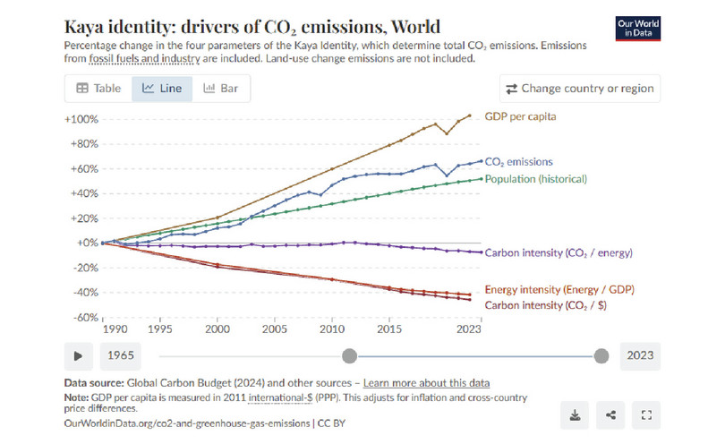
Figure E9.5a Using Kaya’s identity to analyse the drivers of total global CO2 emissions.
| World | 1990 | 2022 | Growth rates (1990–2022) |
|---|---|---|---|
| Population | 5,327,803,039 | 8,021,407,128 | 51% |
| GDP per capita (international $) | 8,210.97 | 16,676.75 | 103% |
| Energy intensity (Wh/international $) | 2.23 | 1.30 | −42% |
| Carbon intensity (ton/Wh) | 0.24 | 0.22 | −7% |
Figure E9.5b Drivers of global CO2 emissions, 1990–2022.
Our World in Data. 2024. Kaya Identity: Drivers of CO2 Emissions, World. Global Carbon Budget.
The data in Figure E9.5a can be interpreted negatively: we have done very little to reduce carbon intensity at a global level, and the modest improvement roughly coincides with the implementation of the Paris agreement. But on the positive side, we still have a policy instrument, greening the generation of energy, almost unused. Therefore, there is room to contain emissions through both efficiency gains and particularly energy transition.
The picture is similar when we compare high-income countries with low- and middle-income countries (Figure E9.5c). The main differences are that high-income countries are more energy-intensive and less carbon-intensive. This is interesting because a few years back, economic greening was almost exclusively happening in high-income countries.8
| High-income countries | 1990 | 2022 | Growth rates (1990–2022) |
|---|---|---|---|
| Population1 | 1,187,952,068 | 1,410,108,183 | 18.7% |
| GDP per capita (international $)2 | 35,231.47 | 56,887.21 | 61.5% |
| Energy intensity (kWh/international $)3 | 1.61 | 0.98 | −39.1% |
| Carbon intensity (kg/kWh)1 | 0.22 | 0.18 | −17.3% |
| Low- and middle-income countries | 1990 | 2022 | Growth rates (1990–2022) |
| Population1 | 4,138,018,604 | 6,608,844,058 | 59.7% |
| GDP per capita (international $)2 | 15,216.97 | 43,848.69 | 188% |
| Energy intensity (kWh/international $)3 | 0.14 | 0.1 | −26.4% |
| Carbon intensity (kg/kWh)1 | 0.83 | 0.74 | −10.3% |
Figure E9.5c Drivers of global CO2 emissions using Kaya’s identity, 1990–2022, for high-income and low- and middle-income countries.
(1) Our World in Data. 2024. Kaya Identity: Drivers of CO2 Emissions, World. Global Carbon Budget. (2) Our World in Data. 2025. GDP Per Capita. Eurostat, OECD, and World Bank Group. (3) Our World in Data. 2024. Kaya Identity: Drivers of CO2 Emissions, high-Income Countries. Global Carbon Budget.
Exercise E9.4 Kaya’s identity
- Between 1990 and 2022, the UK achieved a 47.7% reduction in CO2 emissions. In 2022, the UK’s total net greenhouse gas emissions were approximately 313.8 million metric tons of CO2. During the same period, the UK’s GDP per capita increased from approximately $26,189 in 2000 to $38,407 in 2022. This data suggests that while the UK has made significant progress in reducing greenhouse gas emissions, the relationship between economic growth and emissions reduction remains complex.
- Download UK’s data for 1990 and 2022 from Our World in Data9 and decompose the changes in CO₂ emissions into its factors using Kaya’s identity.
- Compute the contributions of each factor and show that Kaya’s identity holds.
- What is your interpretation of the role of the different drivers?
- Kaya’s identity can also be used to estimate the effort needed to achieve a particular target. Suppose we want to reduce emissions to one-third of the 2010 levels by 2030. We expect annual growths of population and GDP per capita to be 1% and 1.5%, respectively. We also expect the use of energy per output (energy intensity) to decrease by 5% per annum. How much does carbon intensity need to fall by 2030?
-
Ritchie, Hannah. 2023. ‘How Much CO2 Can the World Emit While Keeping Warming Below 1.5°C and 2°C?’. Published online at OurWorldinData.org. ↩
-
United Nations Department of Economic and Social Affairs, Population Division. 2024. World Population Prospects 2024: Summary of Results. United Nations. ↩
-
Caroline Hickman et al. 2021. ‘Climate Anxiety in Children and Young People and Their Beliefs About Government Responses to Climate Change: A Global Survey’. The Lancet Planetary Health 5(12): pp. e863–e873. ↩
-
UNDP (2024) What is climate change adaptation and why is it crucial? 30 January. United Nations. ↩
-
Rupert Way, Matthew C. Ives, Penny Mealy, and J. Doyne Farmer. 2022. ‘Empirically Grounded Technology Forecasts and the Energy Transition’. Joule 6(9): pp. 2057–2082. ↩
-
Philippe Aghion, Ralf Martin Benabou, and Alexandra Roulet. 2023. ‘Environmental Preferences and Technological Choices: Is Market Competition Clean or Dirty?’ AER Insights 5(1): pp. 1–20. ↩
-
OECD. 2023. Effective Carbon Rates 2023: Pricing Greenhouse Gas Emissions through Taxes and Emissions Trading. OECD Series on Carbon Pricing and Energy Taxation, OECD Publishing. ↩
-
Our World in Data. 2024. Kaya Identity: Drivers of CO2 Emissions, High-Income Countries. Global Carbon Budget. ↩
-
Our World in Data. Kaya Identity: Drivers of CO2 Emissions, United Kingdom. Global Carbon Budget. ↩
